| 1.6 | 1.5 | 0.25 | 0 |
| 0.8 | 0.0 | 0.00 | 0 |
| 0.0 | 0.5 | 0.00 | 0 |
| 0.0 | 0.0 | 0.25 | 0 |
Lab 7 Assignment — Age-structured Models
Due by 5:00pm on Friday
Answer each of the following questions and upload your Excel file and R script (graduate students only) to ELC. Be sure to show your calculations. Undergraduates do not have to do either exercise in R. However, undergraduates can get 20 bonus points for doing the entire lab in Excel and R.
Exercise I
Imagine a population with 4 age classes. The fecundities are \(f_1=0\), \(f_2=1.0\), \(f_3=1.5\), and \(f_4=1.2\). The survival probabilities are \(s_1=0.8\), \(s_2=0.5\), \(s_3=0.25\), and \(s_4=0.0\). The initial population sizes are \(n_{1,1}=45\), \(n_{2,1}=18\), \(n_{3,1}=11\), \(n_{4,1}=4\).
- Create a Leslie matrix with the vital rates provided above.
- Project the population forward 25 years and plot abundance for each age class and for the total population size. (Graduate students only: Do the projection using matrix multiplication in R with the
%*%operator. See the end of this document for guidance.) - Create another plot of abundance for each age class, but use the logarithmic scale for the y-axis. This can be done by right-clicking on the y-axis and selecting “Format axis”. Choose the logarithmic axis option with base=10.
- Calculate and plot the age-specific growth rates: \(\lambda_{i,t}\). What is the asymptotic growth rate (\(\lambda\)), rounded to 3 decimals places?
- What is the stable age distribution?
- Graduate students only: Compute asymptotic \(\lambda\) and the stable age distribution using the function in R.
Exercise II
Reproductive value (RV) can be used to identify the age class that contributes the most to population growth. The inoculate method is a way of computing RV by doing one projection for each of the age classes.
For each projection, use a population size of 200 individuals, and put all individuals in one of the four age classes. For example, one projection will have \(n_{1,1}=200\), \(n_{2,1}=0\), \(n_{3,1}=0\), \(n_{4,1}=0\). The next projection will have all 200 individuals in the next age class, and so on. For each projection, record the total population size after 50 time steps. Reproductive value is calculated by dividing each projection’s total population size (\(N_t\)) at \(t=50\) by the total population size from the first projection. (As a result, RV will always be 1 for the first age class when using this method).
- Given the following Leslie matrix, calculate the RV of each age class using the inoculate method.
- If you were charged with reintroducing this species back into the wild, and you could only reintroduce one age class, which one would you release to maximize population growth? Why is reproductive value so high for this age class?
- Graduate students only: Compute reproductive value using the
eigenfunction.
Age-structured models in R
This is an example of an age-structured model with 3 age classes. It is just an example – the parameter values are different than the ones in the assignment above.
First, create the projection matrix.
A <- matrix(c(0.0, 1.5, 0.5,  ## The fecundities
              0.5, 0.0, 0.0,  ## The first value is s1
              0.0, 0.9, 0.0), ## The second value is s2
            nrow=3, ncol=3, byrow=TRUE)
A
[,1] [,2] [,3]
[1,] 0.0 1.5 0.5
[2,] 0.5 0.0 0.0
[3,] 0.0 0.9 0.0Set values of initial abundance and prepare to project over 50 years.
years <- 1:50
nYears <- length(years)
n <- matrix(NA, nYears, 3)
n[1,] <- c(100, 50, 25)    ## Initial abundance
Do the projection.
for(t in 2:nYears) {
  n[t,] <- A %*% n[t-1,]   ## Matrix multiplication
}
Visualize it.
matplot(years, n, type="l", pch=16, xlab="Time", ylab="Abundance")
legend(35, 100, c("Age class 1", "Age class 2", "Age class 3"), col=1:3, lty=1:3)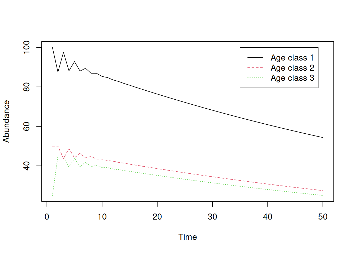
Compute the age distribution and take a look.
N <- rowSums(n) ## Total abundance each year
c <- n/N        ## This works because of R's recycling rules
matplot(years, c, type="l", pch=16, ylim=c(0, 1), xlab="Time",
        ylab="Proportion in each age class")
legend(35, 1, c("Age class 1", "Age class 2", "Age class 3"), col=1:3, lty=1:3)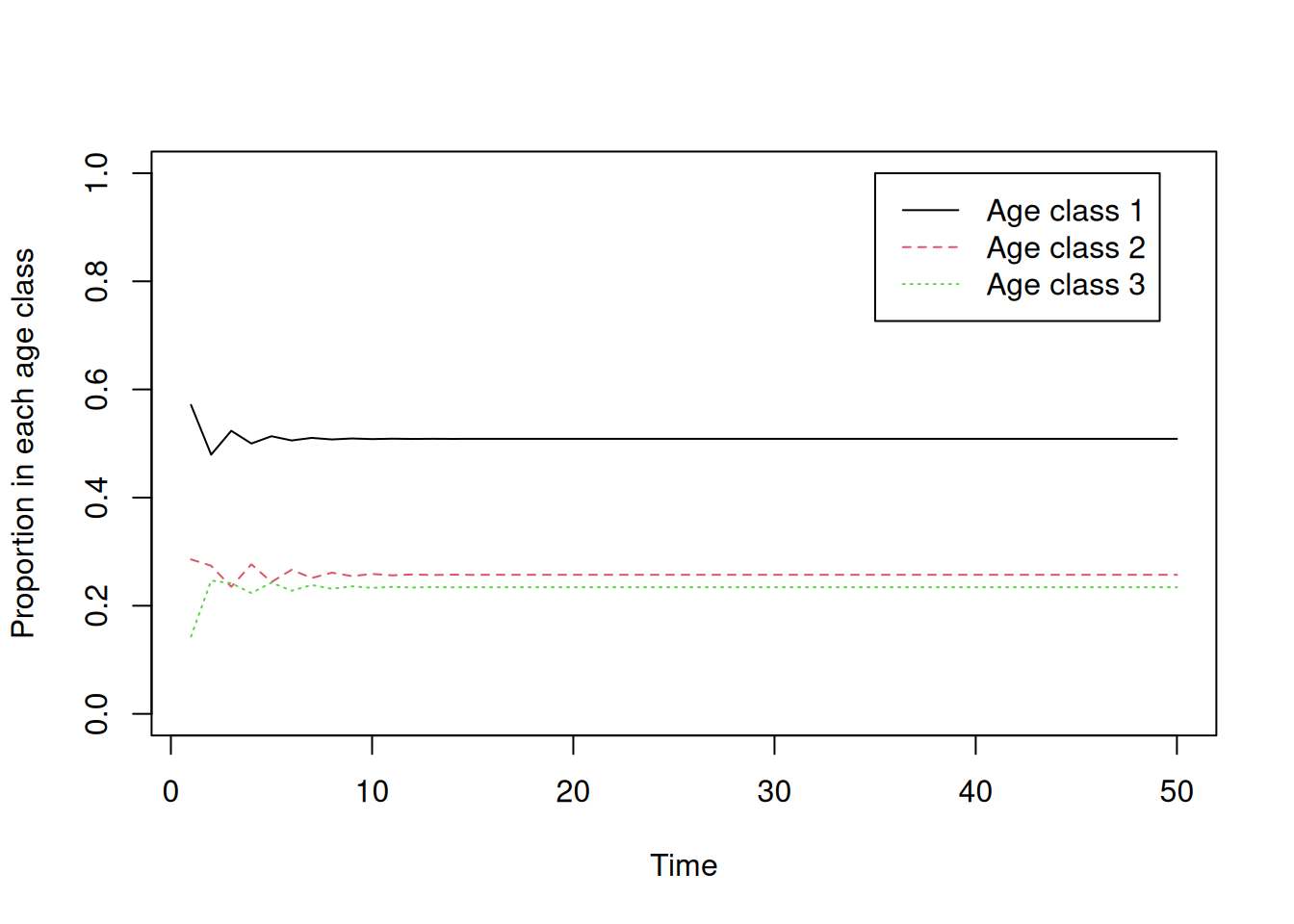
Grab the stable age distribution from the final year.
SAD.proj <- c[nYears,]
SAD.proj
[1] 0.508639 0.257221 0.234140Now compute the annual growth rates for each age class and plot them.
lambda.it <- n[-1,]/n[-nYears,] ## Divide each row by the row before it
matplot(years[-1], ## There are nYears-1 *intervals* between years
        lambda.it, type="l", pch=16, xlab="Time", ylab="Growth rates")
abline(h=1, lty=2, col="grey") ## Horizontal line
legend(35, 1.8, c("Age class 1", "Age class 2", "Age class 3"), col=1:3, lty=1:3)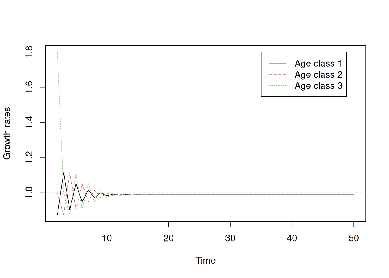
Find asymptotic \(\lambda\) from the last time interval.
lambda.it[nYears-1,] ## These should all be the same[1] 0.9887199 0.9887199 0.9887199lambda.proj <- lambda.it[nYears-1,1]
lambda.proj ## Asymptotic growth rate[1] 0.9887199Now we will use eigenanalysis to compute the growth rate, stable age distribution, and reproductive value.
First compute \(\lambda\).
eA <- eigen(A)
lambda <- Re(eA$values[1])  ## Dominant eigenvalue is the
lambda                      ## asymptotic growth rate
[1] 0.9887199Make sure it’s the same growth rate that we found earlier.
lambda.proj[1] 0.9887199lambda[1] 0.9887199Now find the stable age distribution.
SADu <- Re(eA$vectors[,1])  ## Right eigenvector is stable age dist
SAD <- SADu/sum(SADu)
SAD
[1] 0.508639 0.257221 0.234140Check to make sure that the stable age distribution computed using eigenanalysis is equal to that calculated from the projection.
SAD[1] 0.508639 0.257221 0.234140SAD.proj[1] 0.508639 0.257221 0.234140Now compute the reproductive value (RV) of each age class.
eAT <- eigen(t(A))
RVu <- Re(eAT$vectors[,1]) ## Left eigenvector gives the RVs
RV <- RVu/RVu[1]           ## Standard to divide by first RV
RV
[1] 1.0000000 1.9774397 0.5057044