Answer each of the following questions and upload your completed Excel file and R script to ELC by 5:00pm on Friday. Be sure to show your calculations. Undergrads only need to do the second exercise in R, not the first.
Random Numbers in Excel
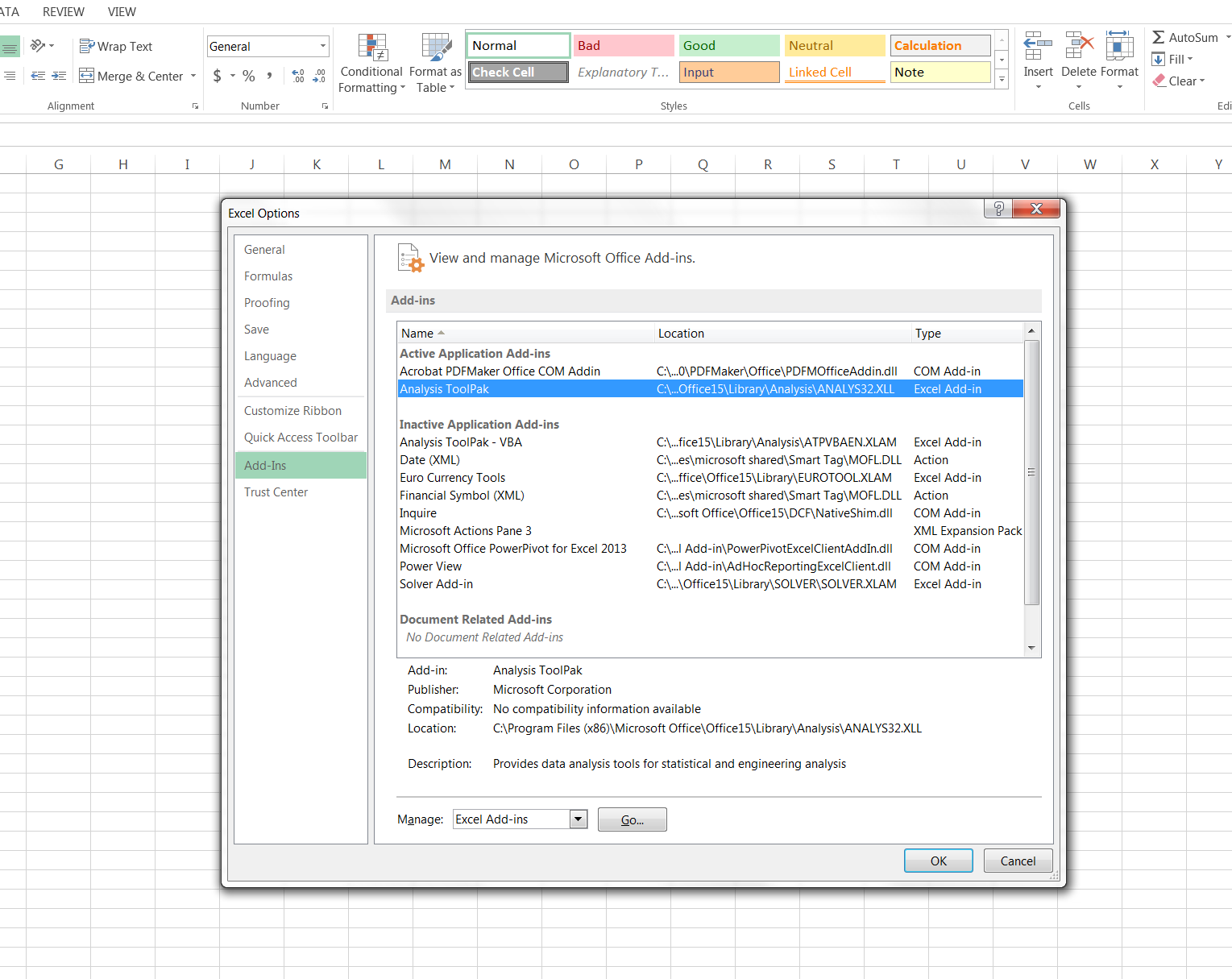
Figure 1: To generate random numbers in Excel, you must load the “Analysis Toolpak” add-in by clicking File > Options > Add-Ins > Analysis Toolpak. Then hit “Go” (not “OK”) and select “Analysis Tookpak” again.
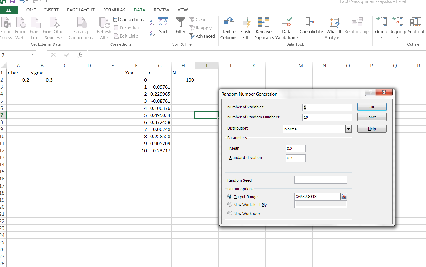
Figure 2: Once the Analysis ToolPak is installed, you can generate random numbers by clicking the “Data Analysis” button in the “Data” tab.
Figure 3: We will use three distributions: Normal, Binomial, and Poisson. The latter two are only used in Exercise II. Note: You can think of the “number of variables” as the number of columns of random variables, and the “number of random numbers” as the number of cells in each column.
Exercise I
Suppose a population is growing geometrically with \(r=-0.2\) and \(N_0=500\). There is no random variation, and quasi-extinction occurs when \(N\) falls below 20 individuals. What is the time to quasi-extinction (\(T_e\))? In other words, how long will it take for the population to fall below 20 individuals?
Now imagine that there is no demographic stochasticity, but environmental stochasticity occurs with \(r_t \sim \mathrm{Normal}(\mathrm{mean}=-0.2, \mathrm{SD}=0.05)\). Generate the random values of \(r_t\) that will be used in the 10 simulations in the next step.
Conduct 10 simulations over a 30 year time period, and force the population size to zero after it falls below the threshold. This can be done by multiplying the geometric growth equation by a “test statement”, like this: =(EQUATION)*(CELL>20), where EQUATION should be replaced with the population growth equation and CELL should be replaced with the cell reference for abundance at the previous time step. Plot the projections (including the one without stochasticity).
What is the average \(T_e\) based on these 10 simulations?
What is extinction risk at year 15?
Exercise II
Assume that a population is geographically closed such that there is no immigration or emigration. The number of individuals born is a Poisson random variable: \[
B_t \sim \mathrm{Poisson}(N_t \times b)
\] and the number that die each year is a binomial random variable: \[
D_t \sim \mathrm{Binomial}(N_t, d)
\] Abundance is just the number that were alive plus the number that were born, minus the number that died: \[
N_{t+1} = N_t + B_t - D_t
\]
Beginning with \(N_0=300\), conduct one simulation over 5 years, in which \(b=0.3\) and \(d=0.2\). Plot the simulated values of abundance over time. Hint: You have to randomly generate \(B_t\) and \(D_t\) before you can compute \(N_{t+1}\), one year at a time. When simulating \(D_t\) from the binomial distribution, the “number of trials” is the population size.
Do you think this population will reach a stochastic equilibrium? Why or why not? (A stochastic equilibrium occurs when a population fluctuates around a long-term average).
Do another simulation, but this time make the mortality rate (\(d\)) density-dependent according to the model \(d_t = 0.2 + 0.001\times N_t\). Will this population reach a stochastic equilibrium? If so, at what value of abundance does the equilibrium point occur?
Example R code
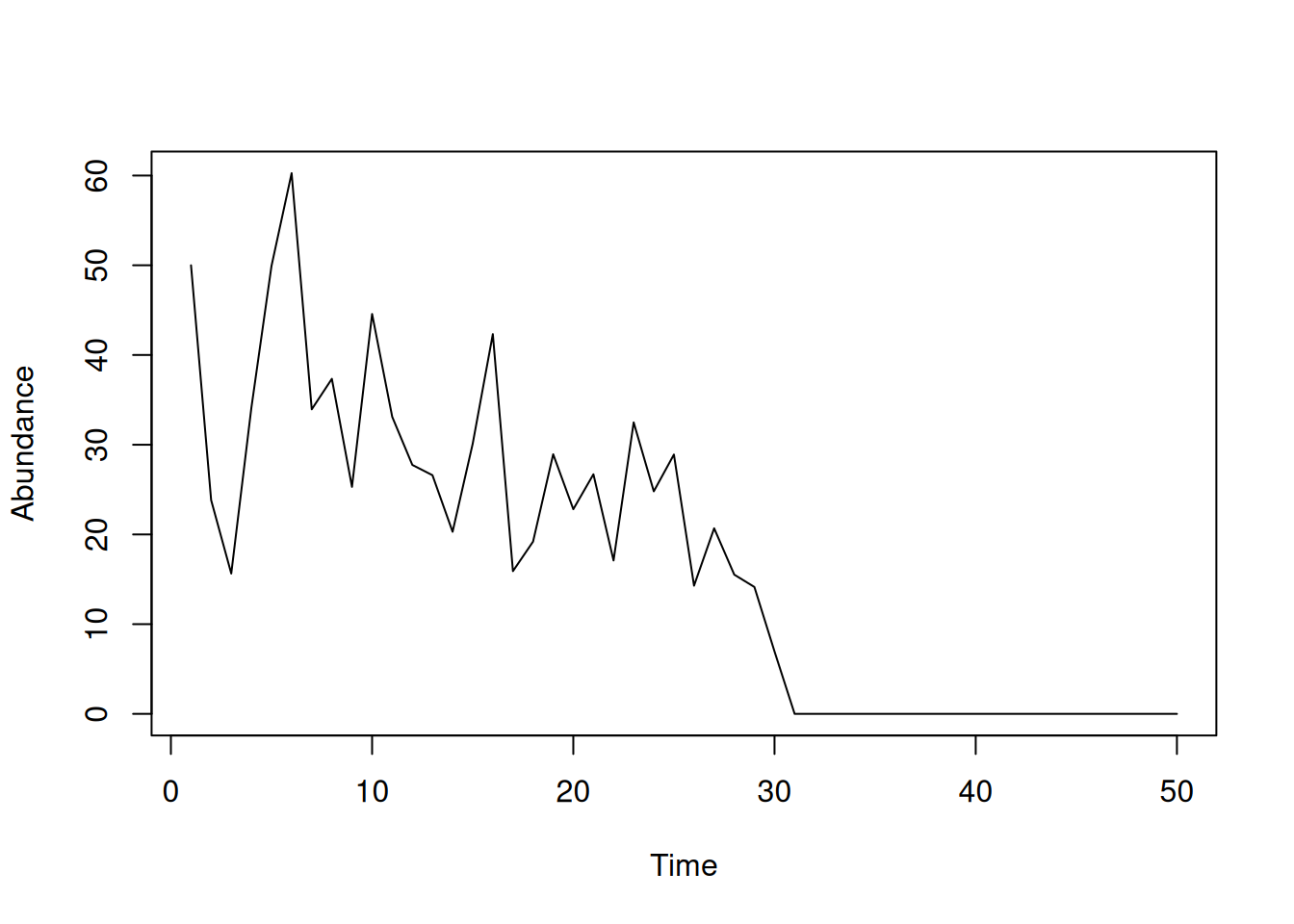
Geometric growth with environmental stochasticity.
rbar <-0sigma <-0.5nYears <-50extinctionThreshold <-10## Repeat the next steps 10 times to do 10 simulations## Or, do a 'nested for loop' and save each simulation (harder)N1 <-rep(NA, nYears) ## Population size N1[1] <-50## Initial population sizer <-rep(NA, nYears-1)for(t in2:nYears) { r[t-1] <-rnorm(n=1, mean=rbar, sd=sigma) # Growth rate from normal distribution N1[t] <- (N1[t-1] + N1[t-1]*r[t-1])*(N1[t-1]>extinctionThreshold)}plot(1:nYears, N1, xlab="Time", ylab="Abundance", type="l")
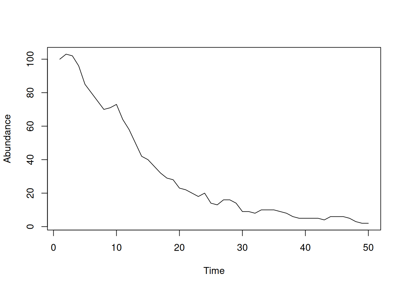
Poisson-Binomial birth-death model.
b <-0.15## Birth rated <-0.2## Mortality ratenYears <-50N2 <-rep(NA, nYears) ## Empty vector for population size B <-rep(NA, nYears) ## Random variable for nBirthsD <-rep(NA, nYears) ## Random variable for nDeathsN2[1] <-100## Initial population sizefor(t in2:nYears) { B[t-1] <-rpois(n=1, lambda=N2[t-1]*b) # Poisson births D[t-1] <-rbinom(n=1, size=N2[t-1], prob=d) # Binomial deaths N2[t] <- N2[t-1] + B[t-1] - D[t-1]}plot(1:nYears, N2, xlab="Time", ylab="Abundance", type="l")