Lab 2 assignment — Geometric growth models Due by 5:00pm on Friday
Answer the following questions by completing the provided Excel template and by replicating your work in R. Undergraduates should do Exercise 1 in R, but not Exercise 2. Graduate students should do both exercises in R. Upload your Excel file and a single R script to ELC. Name the files with your last name followed by your first name.
Exercise 1
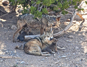
A study was conducted in which a population of 100 Mexican wolves (Canis lupus baileyi) was monitored intensively for 1 year. In that time, 10 pups were born, and 20 of the original 100 individuals died. There was no immigration or emigration.
What are the values of \(B\), \(D\), \(b\), \(d\), \(r\), and lambda (\(\lambda\))?
Assuming geometric growth, what will population size be in each of the subsequent 10 years? Create a graph of the results, including important chart elements such as axis titles. Remember, the geometric growth model is: \(N_{t+1} = N_t + N_t r\).
Exercise 2
Many people assume that the human population acts differently than most wildlife populations and is increasing at an exponential rate, or close to it. The UN estimated that the human population was approximately 7.02 billion in 2010, and 7.11 billion in 2011.
Given these two years of data and the geometric growth equation: \(N_{t+1} = N_t + N_t r\), calculate \(r\) for the human population.
Use the geometric growth equation with the value of \(r\) that you calculated above to predict the human population from 2012 to 2025.
Graph your predictions of the human population along with the actual human population over time.1
Calculate the growth rate lambda (\(\lambda_t = N_t / N_{t-1}\)) for each year and for both the predicted human population and the actual human population data. Graph both values of lambda from 2011 to 2025.
Based on these results, did the human population exhibit geometric growth? Write 2-3 sentences to defend your answer.
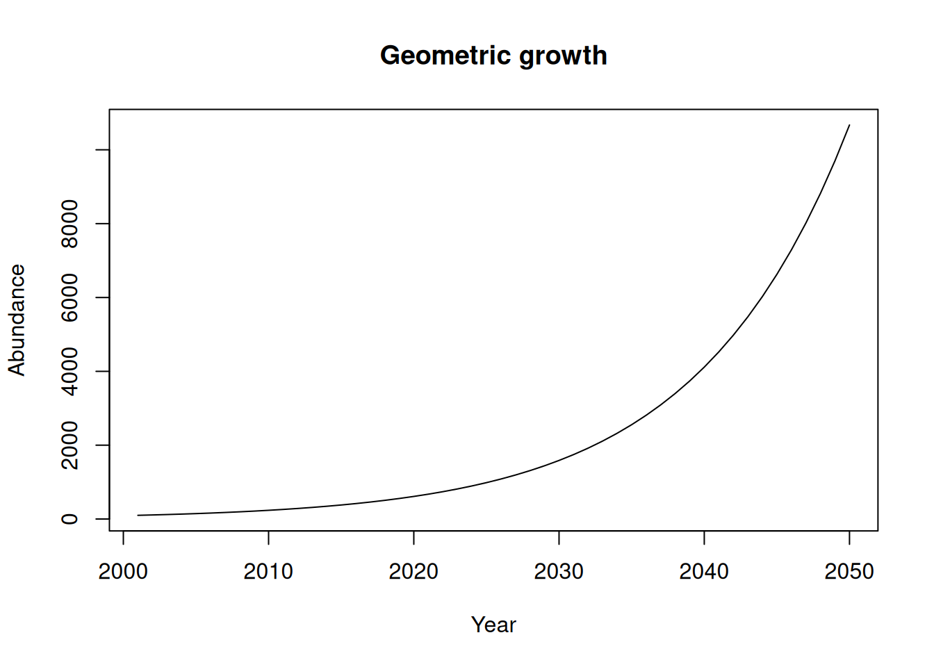
r <-0.1# growth rateyears <-2001:2050# yearsnYears <-length(years) # number of yearsN <-rep(NA, nYears) # empty vectorN[1] <-100# abundance in first yearfor(t in2:nYears) { N[t] <- N[t-1] + N[t-1]*r }plot(years, N, type="l", xlab="Year", ylab="Abundance",main="Geometric growth")
Footnotes
Graduate students, you can import the human population data into R using this code: humans <- c(7.02, 7.11, 7.20, 7.29, 7.38, 7.47, 7.56, 7.65, 7.73, 7.81, 7.89, 7.95, 8.02, 8.09, 8.16, 8.23)↩︎