rmax <- 0.1              ## max growth rate
K <- 200                 ## carrying capacity
years <- 2001:2050       ## years
nYears <- length(years)
N1 <- rep(NA, nYears)
N1[1] <- 100             ## abundance in first year
for(t in 2:nYears) {
    N1[t] <- N1[t-1] + N1[t-1]*rmax*(1 - N1[t-1]/K)
}Lab 3 Assignment — Harvest Models
Due by Friday 5:00pm
Answer the following questions and upload your completed Excel file and R script to ELC. Be sure to show your calculations. Undergraduates need to do both exercises in Excel, but only Exercise I in R. Graduate students should do both exercises in Excel and R.
Exercise I
Imagine a population of northern bobwhite (Colinus virginianus) that is experiencing logistic growth with \(r_\mathrm{max} = 0.32\), \(K = 2000\), and an initial population size of 100 individuals.
- Project the population for 40 years, and plot abundance over time. Add axis labels as always.
- Compute the number of individuals that could be sustainably harvested each year. Plot abundance on the x-axis and sustainable harvest on the y-axis.
- At what value of abundance (\(N\)) would maximum sustainable yield (MSY) occur?
- What is the value of MSY in this case? In other words, what is maximum number of individuals that can be sustainably harvested?
- Using the same values of \(r_\mathrm{max}\), \(K\), and \(N_0\), project the population forward again, but include harvest (\(H_t\)) in the model. Choose values of \(H_t\) that allow for the greatest number of years at MSY. Hint: You can let harvest be zero in some years.
Exercise II
Suppose that annual survival of sitka deer (Odocoileus hemionus sitkensis) decreases as abundance increases according to the equation: \(S = \beta_0 - \beta_1 \times N\).
- Compute survival probability for each value of \(N\) provided in the spreadsheet with \(\beta_0=0.95\) and \(\beta_1=0.003\). Create a graph with survival probability on the y-axis and abundance on the x-axis.
- A manager is trying to decide how many deer to harvest, and is considering removing anywhere from 10 to 150 individuals from a population of 200. Use the equation above to determine how many deer will remain one year after harvest for each of the harvest options. To accomplish this, do the following:
- Compute how many individuals will be alive immediately after harvest (Hint: You just have to subtract \(H\) from \(N=200\));
- Compute survival probability for these remaining individuals using the survival equation above;
- Compute how many will be alive at the end of the year. In other words, what fraction of the individuals after harvest will survive and be alive next year?
- Create a graph with final abundance (\(N\)) on the y-axis and harvest (\(H\)) of the x-axis.
- Determine how many deer will be alive if no harvest occurs. Are there any levels of harvest that can result in a larger population than the “no harvest” scenario? If so, how can this be?
- If the manager’s objective is to maximize harvest, while maintaining a herd size greater than it would be without harvest, how many deer should be taken?
R tips
Here’s an example of a logistic growth model.
Here’s an example of a logistic growth model with harvest
h <- 0.02                ## harvest rate (not the sustainable harvest rate)
N2 <- rep(NA, nYears)
N2[1] <- 100             ## abundance in first year
H <- rep(NA, nYears-1)
for(t in 2:nYears) {
    H[t-1] <- N2[t-1]*h  ## harvest
    N2[t] <- N2[t-1] + N2[t-1]*rmax*(1 - N2[t-1]/K) - H[t-1]
}
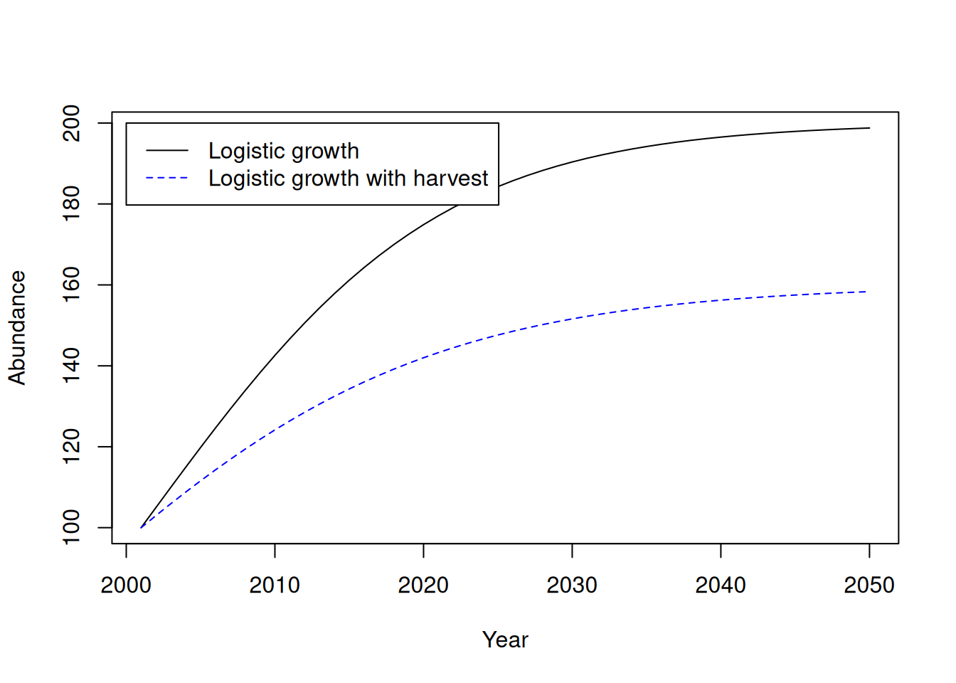
plot(years, N1, type="l", xlab="Year", ylab="Abundance")
lines(years, N2, col="blue", lty=2)
legend(2000, 200, c("Logistic growth", "Logistic growth with harvest"),
       col=c("black", "blue"), lty=c(1,2))