Lab 6 Assignment — Models of Interspecific Interactions Due by 5:00pm on Friday
Answer each of the following questions and upload your Excel file and R script to ELC. Be sure to show your calculations. Undergraduates only have to do Exercise I in R.
Exercise I
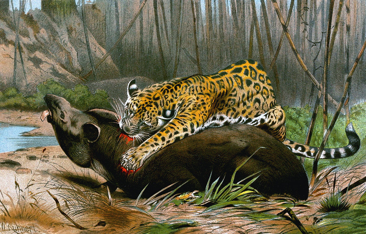
You are studying the dynamics of jaguar (Panthera onca) and Baird’s tapir (Tapirus bairdii) in Costa Rica’s Corcavodo National Park. After years of research, you obtain the following parameter estimates, which you would like to use in a Lotka-Volterra model: \(r^{prey}=0.05\), \(k^{pred}=0.0005\), \(b^{pred}=0.001\), and \(d^{pred}=0.45\).
What predator population size corresponds to prey equilibrium? What prey population size corresponds to predator equilibrium?
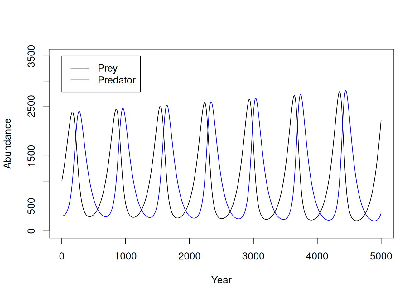
Project the populations 100 years following an initial prey population size of \(N_0^{prey}=500\) and an initial predator population size of \(N_0^{pred}=100\). Plot the projections.
Clearly, these populations have not reached a stable equilibrium, so what is the interpretation of the equilibrium values from part (a)? What happens if you set the initial population sizes to the equilibrium values?
Exercise II
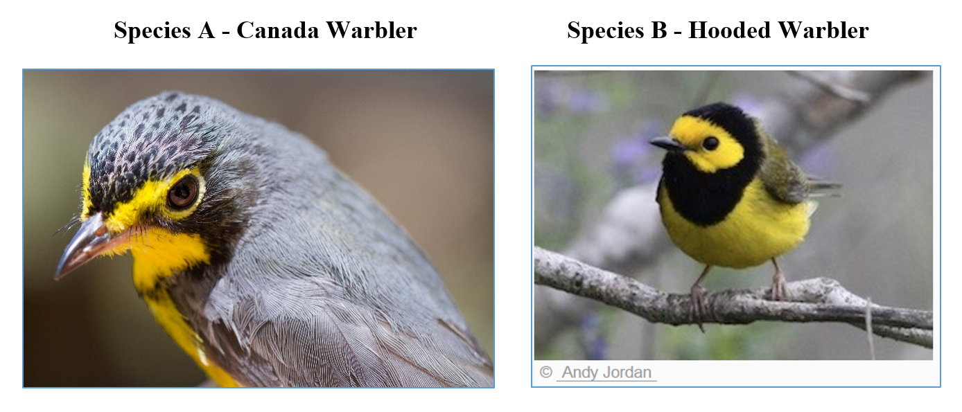
The Canada warbler (Cardellina canadensis) and the hooded warbler (Stetophaga citrina) are two species of Neotropical-Nearctic migratory birds that appear to compete for the same resources where their ranges meet in the southern Appalachian Mountains. Assume their dynamics follow the Lotka-Volterra competition model with parameters \(r^{A}=0.2\), \(r^{B}=0.3\), \(K^{A}=250\), \(K^{B}=200\), \(\alpha^{A}=0.1\), and \(\alpha^{B}=0.1\).
Plot 25 years of dynamics following initial conditions of \(N_0^A = 200\) and \(N_0^B=50\).
What are the 2 equilibrium values for these species?
Do these conditions describe stable coexistence, competitive exclusion, or unstable equilibrium?
What is the minimum value of \(\alpha^B\) that would result in competitive exclusion of species A? (Hint: Use the equilibrium equations to solve for \(\alpha^B\)). Plot 25 years of dynamics under this scenario. Use the same initial abundance values as before.