install.packages("unmarked")Lab 9 Assignment — Occupancy Models in R
Due by 5:00pm on Friday
Answer each of the following questions, and submit your answers by uploading a single WORD file to ELC. Unlike previous labs, copy and paste code and results from R to the WORD file. You should also copy and paste entire screenshots to show the relevant output. If you know how to use RMarkdown or Quarto, please do so.
Preliminaries: Occupancy models using the R package ‘unmarked’
Occupancy models can be fit using the ‘unmarked’ package in R. To install ‘unmarked’, issue this R command:
Once it’s installed, you need to load it:
library(unmarked)Getting Data into R
Now we’re ready to import the data. For exercise I, you will import the file named
quail-data-for-R.csv. For exercise II, you will import the file dipnet-data-for-R.csv. Before you import those files, here is some general guidance on importing data, followed by occupancy modeling examples.
The easiest way to import data into R is to save the data as a .csv file, which has been done for you already, and put it in your working directory. The working directory is the location on your computer where R will look for files by default. To find out where the working directory is, do this:
getwd()If getwd() returns the location where you put your data, then you are ready to import. Otherwise, you need to change your working directory to the location where your data files are located. You can change your working directory using the setwd command or using the drop-down menu options (Session > Set Working Directory).
Once your working directory is correctly specified, you can import the data using this command:
exampleData <- read.csv("example-data.csv")Let’s look at a summary:
summary(exampleData) Site season1visit1 season1visit2 season2visit1 season2visit2 habitatIndex
Min. : 1.00 Min. :0.0 Min. :0.000 Min. :0.0 Min. :0.00 Min. :1.040
1st Qu.:10.75 1st Qu.:0.0 1st Qu.:0.000 1st Qu.:0.0 1st Qu.:0.00 1st Qu.:1.885
Median :20.50 Median :0.0 Median :0.000 Median :0.0 Median :0.00 Median :2.805
Mean :20.50 Mean :0.4 Mean :0.325 Mean :0.3 Mean :0.25 Mean :2.912
3rd Qu.:30.25 3rd Qu.:1.0 3rd Qu.:1.000 3rd Qu.:1.0 3rd Qu.:0.25 3rd Qu.:3.835
Max. :40.00 Max. :1.0 Max. :1.000 Max. :1.0 Max. :1.00 Max. :4.740 Columns 2-5 have the occupancy data. The sixth column has a site-specific covariate. Before we can run a single-season occupancy model, we have to format the data.
Example: Formatting data for single-season analysis in ‘unmarked’
The example dataset is from a study with 2 seasons, but we’ll begin by pretending that it is from a single season with 4 surveys at each site.
## First, extract columns 2-4 with the occupancy data
occData <- exampleData[,c("season1visit1", "season1visit2",
                          "season2visit1", "season2visit2")]
## Next, extract the column with the site covariate.
## It must be formatted as a data.frame
habIndex <- exampleData[,"habitatIndex",drop=FALSE]
## Finally, put the pieces together
umf <- unmarkedFrameOccu(y=occData, siteCovs=habIndex)
Now that we have the data formatted, we should summarize it again to make sure everything looks good:
summary(umf)unmarkedFrame Object
40 sites
Maximum number of observations per site: 4
Mean number of observations per site: 4
Sites with at least one detection: 22
Tabulation of y observations:
0 1
109 51
Site-level covariates:
habitatIndex
Min. :1.040
1st Qu.:1.885
Median :2.805
Mean :2.912
3rd Qu.:3.835
Max. :4.740 All is well. Let’s fit some models.
Example: Fitting single-season occupancy models
Model fitting is the process of fitting a model to the data. In other words, it is the process of estimating the parameters of a model using a dataset.
We will fit two models using the occu function. In the first model, there are no covariates, meaning that occupancy probability (\(\psi\)) and detection probability (\(p\)) are constant. We will call this the null model:
nullModel <- occu(~1 ~1, umf)The line of code above fits the single-season model to the data. The first argument is a formula describing the model that you want to fit. If the formula is ~1 ~1, then there are no covariates. If there are covariates, the detection probability covariates go after the first ~ and the occupancy covariates go after the second ~. We will add covariates later. First, let’s summarize the results:
summary(nullModel)
Call:
occu(formula = ~1 ~ 1, data = umf)

Occupancy (logit-scale):
 Estimate    SE     z P(>|z|)
     0.29 0.338 0.858   0.391

Detection (logit-scale):
 Estimate    SE     z P(>|z|)
     0.23 0.235 0.977   0.328

AIC: 177.2621
Number of sites: 40
Notice that the parameters are estimated on the logit-scale. To get estimates on the probability scale, we need to back-transform them. If there are no covariates, we can back-transform like this:
## Occupancy estimate - Pr(site is occupied)
backTransform(nullModel, type="state")
Backtransformed linear combination(s) of Occupancy estimate(s)
Estimate SE LinComb (Intercept)
0.572 0.0827 0.29 1
Transformation: logistic ## Detection probability estimate
backTransform(nullModel, type="det") Backtransformed linear combination(s) of Detection estimate(s)
Estimate SE LinComb (Intercept)
0.557 0.0581 0.23 1
Transformation: logistic We conclude that the probability that a site is occupied is 0.572. The probability that the species is detected (on a single visit), if the site is occupied, is 0.557. These two estimates are similar, but that is just a coincidence.
Let’s now assess the possibility that occupancy probability depends on the habitat index. We can fit such a model like this:
detNullOccHab <- occu(~1 ~habitatIndex, umf)The summary indicates that habitat effect is positive, indicating that occupancy probability increases as the index increases.
summary(detNullOccHab)
Call:
occu(formula = ~1 ~ habitatIndex, data = umf)

Occupancy (logit-scale):
             Estimate    SE     z P(>|z|)
(Intercept)    -1.768 1.017 -1.74  0.0820
habitatIndex    0.723 0.348  2.08  0.0378

Detection (logit-scale):
 Estimate    SE     z P(>|z|)
     0.23 0.235 0.979   0.327

AIC: 174.192
Number of sites: 40
To visualize the habitat effect, we need to predict occupancy at several values of the habitat index, which ranged in value from approximately 1–5. We can create a sequence of values and put it into a data frame for prediction like this:
predData <- data.frame(habitatIndex=seq(from=1, to=5, length.out=10))Now, let’s do the prediction:
predOcc <- predict(detNullOccHab, newdata=predData, type="state", append=TRUE)
predOcc
Predicted SE lower upper habitatIndex
1 0.2601584 0.13530441 0.08144029 0.5824030 1.000000
2 0.3265380 0.12675690 0.13544954 0.6000900 1.444444
3 0.4006819 0.11216471 0.21113434 0.6254747 1.888889
4 0.4796701 0.09729524 0.30039695 0.6643364 2.333333
5 0.5596880 0.09008114 0.38307019 0.7223861 2.777778
6 0.6367200 0.09342213 0.44264168 0.7945805 3.222222
7 0.7073227 0.10152150 0.48032215 0.8633721 3.666667
8 0.7691782 0.10736889 0.50459780 0.9159817 4.111111
9 0.8212643 0.10774837 0.52155057 0.9509032 4.555556
10 0.8636800 0.10262384 0.53440045 0.9722013 5.000000The “Predicted” values are the estimates of occupancy for each value of “habitatIndex”. Standard errors and 95% confidence intervals are also returned. Here’s how to visualize the predictions with the confidence intervals:
plot(Predicted ~ habitatIndex, data=predOcc, type="l", ylim=c(0,1),
     xlab="Habitat index", ylab="Occupancy")
lines(lower ~ habitatIndex, data=predOcc, lty=2)
lines(upper ~ habitatIndex, data=predOcc, lty=2)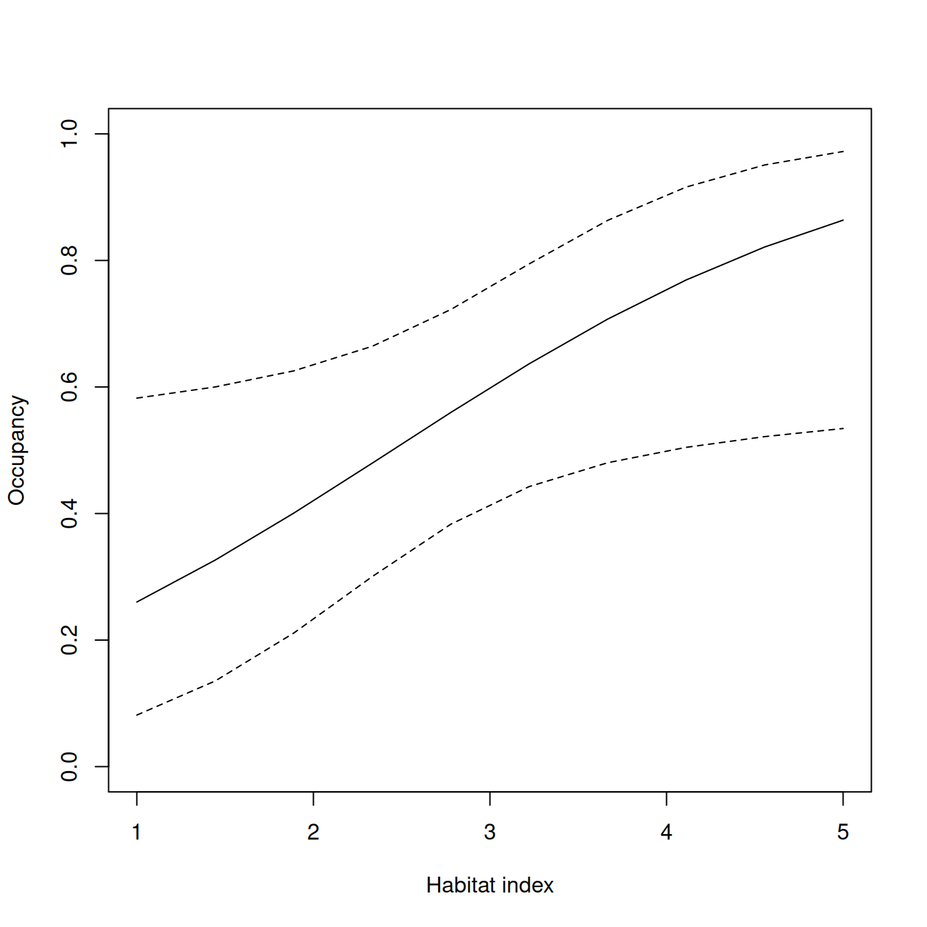
Example: Fitting multi-season occupancy models
We will use different functions to format the data and fit the multi-season occupancy models. Instead of using unmarkedFrameOccu, we will use unmarkedMultFrame. The number of seasons must be specified using the numPrimary argument.
umfMS <- unmarkedMultFrame(y=occData, numPrimary=2)Let’s take a look.
summary(umfMS)unmarkedFrame Object
40 sites
Maximum number of observations per site: 4
Mean number of observations per site: 4
Number of primary survey periods: 2
Number of secondary survey periods: 2
Sites with at least one detection: 22
Tabulation of y observations:
0 1
109 51 Model fitting is done using the colext function instead of the occu function. Notice that the formulas have spaces between them, unlike before.
nullModelMS <- colext(~1, ~1, ~1, ~1, umfMS)Here are the results:
summary(nullModelMS)
Call:
colext(psiformula = ~1, gammaformula = ~1, epsilonformula = ~1,
    pformula = ~1, data = umfMS)

Initial (logit-scale):
 Estimate    SE     z P(>|z|)
    0.207 0.401 0.516   0.606

Colonization (logit-scale):
 Estimate   SE    z P(>|z|)
    -2.78 2.31 -1.2   0.229

Extinction (logit-scale):
 Estimate    SE     z P(>|z|)
    -1.35 0.829 -1.63   0.103

Detection (logit-scale):
 Estimate    SE    z P(>|z|)
    0.521 0.339 1.54   0.124

AIC: 178.8779
Number of sites: 40
We can back-transform and predict as before, but should be one of: “psi”, “col”, “ext”, or “det”.
backTransform(nullModelMS, type="psi")Backtransformed linear combination(s) of Initial estimate(s)
Estimate SE LinComb (Intercept)
0.552 0.0992 0.207 1
Transformation: logistic backTransform(nullModelMS, type="col")Backtransformed linear combination(s) of Colonization estimate(s)
Estimate SE LinComb (Intercept)
0.0586 0.127 -2.78 1
Transformation: logistic backTransform(nullModelMS, type="ext")Backtransformed linear combination(s) of Extinction estimate(s)
Estimate SE LinComb (Intercept)
0.206 0.135 -1.35 1
Transformation: logistic backTransform(nullModelMS, type="det")Backtransformed linear combination(s) of Detection estimate(s)
Estimate SE LinComb (Intercept)
0.627 0.0793 0.521 1
Transformation: logistic The occupancy estimate is associated with the first season.
Exercise I: Single-season models
Suppose we are interested in estimating occupancy of bobwhite quail (Colinus virginianus) in abandoned ag fields. We randomly select 50 sites and survey them 4 times each in May. The resulting data indicate whether at least one quail was detected at each site on each visit.
In addition, you think there is a possibility that vegetation height affects both occupancy and detection probability so you measure average vegetation height at each site. Vegetation height will be the covariate used in the analysis.
Import the file quail-data-for-R.csv.
- Fit the single-season null model using the
occufunction. Report the estimates and standard errors for psi (\(\psi\)) and \(p\) (on the probability scale). Interpret these estimates (ie, what are the definitions of \(\psi\) and \(p\) in this context?). - Now run another model using
veghtas a predictor variable (covariate) for both occupancy and detection probability. - Is this model better than the first, based on AIC? The lower the AIC, the better the model’s predictive performance.1 AIC favors models that explain a lot of variation in the data using a small number of parameters.
- Use the model to create a graph of the relationship between occurrence probability and vegetation height. Do this using the
predictfunction as described above. Add the graph to your Word document.
Exercise II: Multi-season model
Use the southern two-lined salamander (Eurycea cirrigera) data from the past few years to do the following. Note: I pooled the data from the 5 swipes of each team.
Begin by importing the file dipnet-data-for-R.csv.
- Use the
colextfunction to fit the null multi-season occupancy model. Report the estimates and standard errors for psi (\(\psi\)), gamma (\(\gamma\)), epsilon (\(\epsilon\)), and \(p\) on the probability scale. Report these values in a table in your Word document. - Provide clear interpretations of the estimates.
- Based on these estimates, is there any reason to believe that occupancy has decreased over these years? Explain.
- How certain are you of these conclusions? Answer by describing how well you think our study design met the assumptions of the multi-season occupancy model.
Footnotes
AIC = \(-2\times \mathrm{log(likelihood)} + 2\times \mathrm{nParameters}\).↩︎