Capture-mark-recapture methods for abundance estimation

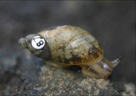
Abundance estimation

Same old equation:

\[ \hat{N} = \frac{n}{\hat{p}} \]

\(N\) is abundance (population size)
\(n\) is the number of individuals detected
\(\hat{p}\) is an estimate of detection probability: The probability of detecting an individual

Most methods differ in how they estimate \(p\)

Overview

Estimating \(p\)

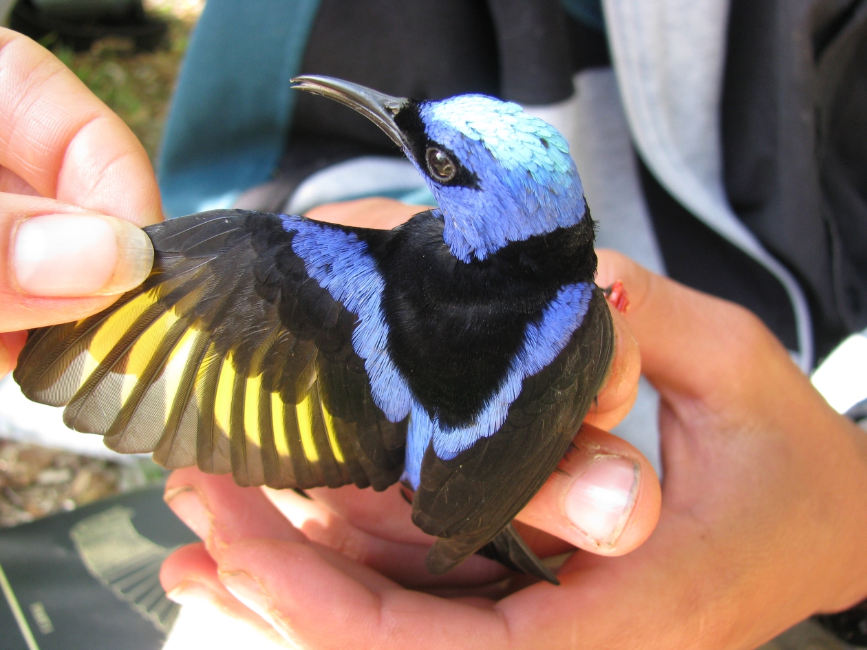
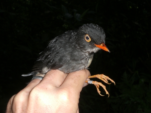
Set traps in a study area and mark each captured individual
Repeat the trapping on \(K\) occasions
On each occasion, mark new individuals and record recaptures
If capture probability is high…
- You will detect most of the population on the first occasion
- Most of the captures on subsequent occasions will be recaptures
And vice versa

Encounter histories

\(n=5\) individuals captured over 3 sampling occasions

Individual	Occasion 1	Occasion 2	Occasion 3
1	0	0	1
2	1	1	0
3	1	1	1
4	1	0	0
5	0	1	0

These data tell us about \(p\) and hence \(N\). Estimation is usually acheived using maximum likelihood methods.

Lincoln-Peterson

Lincoln-Peterson Method

The original method was first used by Pierre-Simon LaPlace to estimate the human population in France.

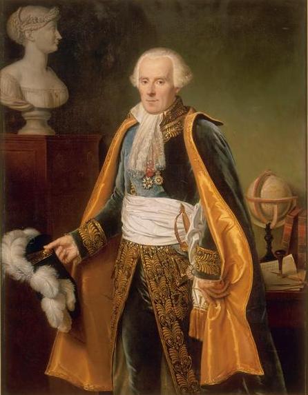
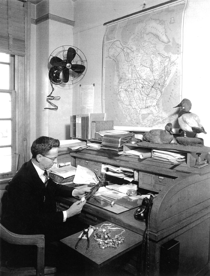
Later it was used by Lincoln (shown above) and Peterson to estimate fish and wildlife populations.

Lincoln-Peterson Study Design

There are only 2 capture occasions
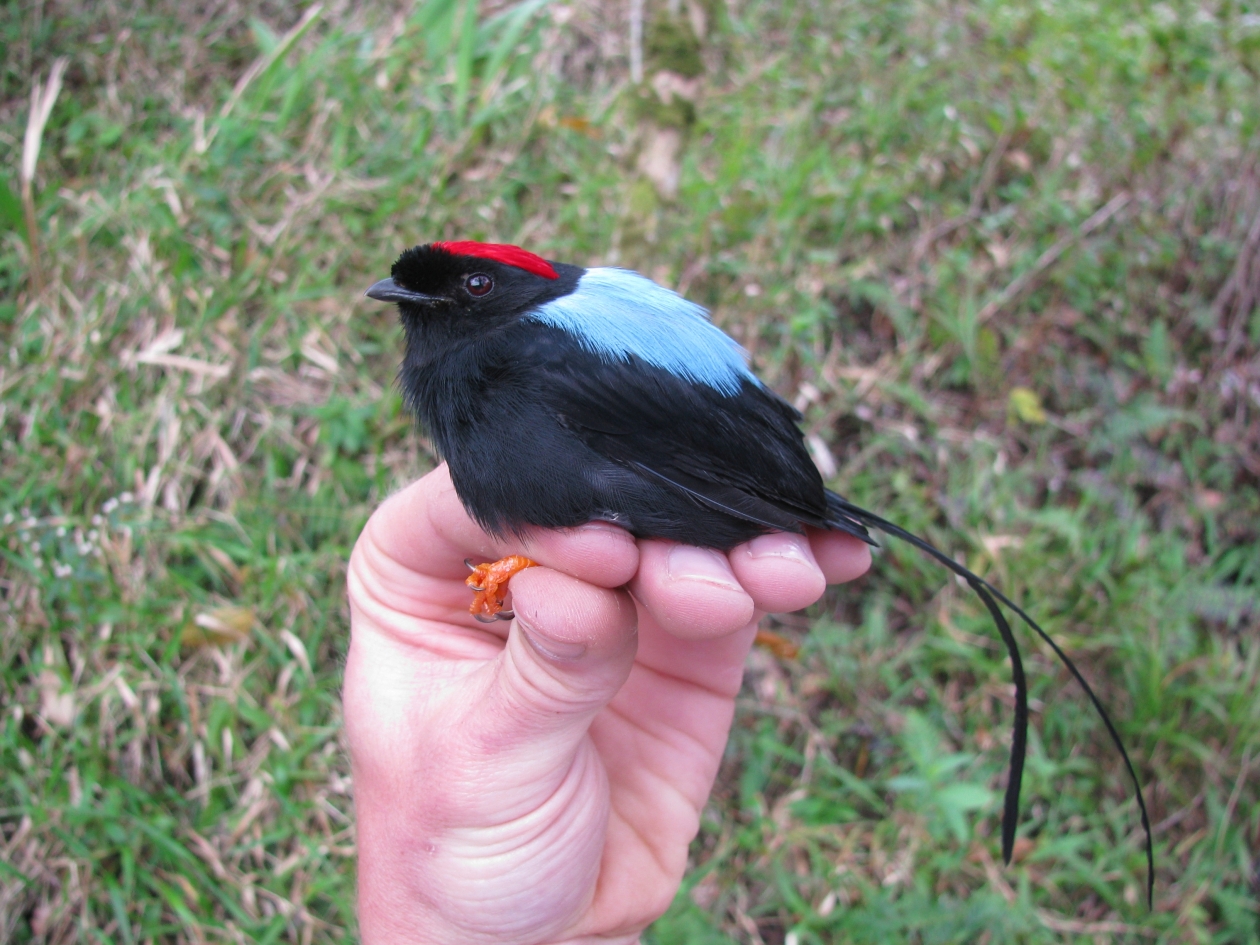
On the first, \(n_1\) animals are captured and marked
On the second, \(n_2\) animals are captured and \(m_2\) of them are recaptures

Lincoln-Peterson Abundance Estimator

How can we use \(n_1\), \(n_2\), and \(m_2\) to estimate \(N\)?

\[ \frac{n_1}{N} = \frac{m_2}{n_2} \]

And so…

\[ \hat{N} = \frac{n_1n_2}{m_2} \]

Lincoln-Peterson Assumptions

Population closure
- No births
- No deaths
- No immigration or emigration

All individuals are assumed to have the same capture probability

No tag loss or mis-identification

\(K\)-sample CMR

K-sample CMR

Using more than 2 sampling occasions has many advantages, including the ability to account for:

Temporal variation

Behavioral effects
- Trap happiness
- Trap shyness

Individual heterogeneity

Combinations of the above

Common models

Model	Description
\(M_0\)	The most basic model in which \(p\) and \(c\) are constant
\(M_t\)	\(p\) differs among sampling occasions and \(p_t=c_t\).
\(M_b\)	Behavioral response model in which \(p\) and \(c\) differ. Can describe trap happiness or trap shiness.
\(M_{tb}\)	A combination of models \(M_t\) and \(M_b\).

where

\(p =\) capture probability
\(p_t =\) capture probability on occasion \(t\)
\(c =\) recapture probability

Removal sampling

Video

Removal sampling

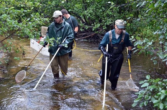
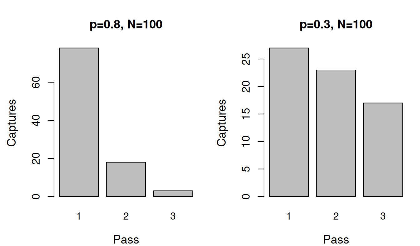
Suppose you conduct several electrofishing passes on a single stream section, and you remove individuals on each pass.

Eventually you should deplete the population.

The number of captures you would expect on each pass:

Pass	Expected captures
1	\(pN\)
2	\(p(1-p)N\)
3	\(p(1-p)^2N\)
4	\(p(1-p)^3N\)
\(\vdots\)	\(\vdots\)
K	\(p(1-p)^{K-1}N\)

Example

The rate at which the population is depleted tells us about \(p\), and therefore how many individuals we missed.

Estimating density

Lingering questions

How do we convert abundance to density?
What is the area surveyed?
How do we model spatio-temporal variation in density?

Summary

Capture-recapture methods use information about recapture rates to estimate capture probability and abundance.

Modern methods use camera traps or DNA sampling techniques to collect non-invasive capture-recapture data and estimate density and vital rates.

Assignment

Read Chapter 11