Mark-recapture methods for estimating survival and recruitment

Accounting for imperfect detection

Suppose we mark and release \(R\) individuals, and then recapture \(m\) of them on the second occasion. How do we estimate survival probability?

If capture probability (\(p\)) was 1, we could use: \[ \hat{S} = \frac{m}{R} \]

But when \(p<1\), \(m\) is some fraction of the number actually alive (\(M\)), so we have to estimate \(p\) and \(M\) to estimate \(S\):

\[ \hat{S} = \frac{\hat{M}}{R} \]

where

\[ \hat{M} = \frac{m}{\hat{p}} \]

Tag recovery models

Tag recovery models

Purpose

Estimate survival from recovered tags.

Benefit

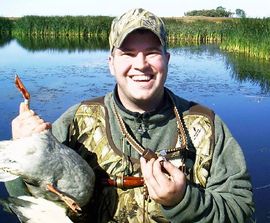
Because hunters are just about everywhere, we don’t have to worry about animals leaving “the study area” and we can estimate actual survival.

Tag recovery models

Design

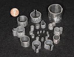
• Animals are marked and released
• Hunters or anglers report tags from harvested individuals
• Desirable to have at least 5 releases

Data

Three release years followed by 3 years of recoveries:

Number released	Period recovered
	1	2	3
\(R_1\)	\(m_{1,1}\)	\(m_{1,2}\)	\(m_{1,3}\)
\(R_2\)		\(m_{2,2}\)	\(m_{2,3}\)
\(R_3\)			\(m_{3,3}\)

Tag recovery models

Expected values

Period released	Number released	Period recovered
		1	2	3
1	\(R_1\)	\(R_1f_1\)	\(R_1S_1f_2\)	\(R_1S_1S_2f_3\)
2	\(R_2\)		\(R_2f_2\)	\(R_2S_2f_3\)
3	\(R_3\)			\(R_3f_3\)

Parameters

• Survival (\(S\))
• Recovery rate (\(f\))

Software programs like “MARK” (and “RMark” and “Rcapture” in R) find the most likely values of \(S\) and \(f\), given the data.

Tag recovery models

Assumptions

• Sample is representative of population
• No tag loss, mis-identification, etc
• All animals have common survival and recovery rates
• Fates are independent

Extensions

• Age-specific models
• Grouping variables
• Time variables
• Habitat variables

Canada goose banding video

Duck banding video

CJS model

Cormack-Jolly-Seber (CJS) model

Purpose

Estimate survival and capture probability from capture-recapture data.

Design

A random sample of animals is marked and followed over many periods (eg, years).

Notes

• When permanent emigration is possible, we can’t be sure if an animal died or left study area
• So we often have to estimate apparent survival (\(\Phi\)) instead of actual survival (\(S\))
• Apparent survival is the probability that an individual survives and does not permanently emigrate out of the study area

CJS capture histories

In CJS studies, we ignore the leading zeros in the capture histories because we aren’t interested in how animals enter the sample.

All we care about is survival, so we “condition” on first encounter.

	Year 1	Year 2	Year 3
Animal 1	1	0	0
Animal 2		1	0
Animal 3			1
Animal 4	1	1	1
Animal 5		1	1

CJS capture histories

Estimation is accomplished by finding the values of \(p\) and \(\Phi\) that best align the expected values with the observed capture histories.

Capture history	Expected values
111	\(\Phi_1p_2\Phi_2p_3\)
110	\(\Phi_1p_2(1-\Phi_2p_3)\)
101	\(\Phi_1(1-p_2)\Phi_2p_3\)
100	\((1-\Phi_1)+\Phi_1(1-p_2)(1-\Phi_2p_3)\)

CJS model

Assumptions

• Same as tag-recovery, plus
• Instantaneous recapture and release of animals
• Homogeneity of capture and survival probabilities for marked animals
• All emigration is permanent

Model can be extended to accommodate variation due to…

• Age
• Sex
• Habitat
• Geographical regions

JS model

Jolly-Seber (JS) model

Purpose

Estimate survival, recruitment, abundance, and capture probability from capture-recapture data.

Design

Randomly sample the population during every period and mark all newly captured unmarked animals.

Examples

• Constant-effort mist-netting
• Long-term small mammal trapping

Recruitment in the Jolly-Seber model

Recruitment in JS models is defined as the per-capita rate at which new individual enter the population.

If immigration is not possible, recruitment is equivalent to fecundity.

Note that in other applications, recruitment is defined as the product of the birth rate and the probability of surviving to maturity.

JS capture histories

We no longer “condition” on first encounter – Instead, we use all the data.

The leading zeros provide information about when individuals are recruited into the population.

	Year 1	Year 2	Year 3
Animal 1	1	0	0
Animal 2	0	1	0
Animal 3	0	1	1
Animal 4	1	1	1
Animal 5	0	1	1

Jolly-Seber model

Assumptions

• All the assumptions of CJS model, plus…
• Every animal — marked or unmarked — has the same probability of capture

The standard JS model doesn’t work very well, but it is extremely powerful when combined with the robust design.

Robust design

Robust design

Purpose

Relax assumptions and increase precision by collecting more data.

Key concept

We now have two types of sampling periods:

• Primary sampling periods: the population is assumed to be open
• Secondary sampling periods:the population is assumed to be closed

The replicate surveys with each primary period give us direct information about capture probability, which makes it easier to estimate the other parameters.

Robust design capture histories

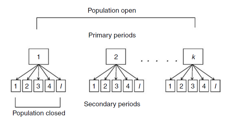
Example with 2 primary periods and 3 secondary periods:

	Primary period 1				Primary period 2
2-4	Day 1	Day 2	Day 3		Day 1	Day 2	Day 3
Animal 1	0	0	1		1	0	0
Animal 2	1	0	1		1	1	1
Animal 3	0	0	0		1	0	0
Animal 4	1	1	1		0	0	0
Animal 5	0	0	0		1	1	0

Summary

Method	Data	Survival	Recruitment	Abundance
Tag recovery	Recoveries	Yes	No	No
CJS	Mark-recap	Yes\(^1\)	No	No
JS	Mark-recap	Yes\(^1\)	Yes	Yes

Each of these three methods is widely used in practice. The best option depends on the objectives.

\(^1\) Apparent survival