Distance sampling
Design
- Randomly place line transects or points throughout the study area
- Record the distance to each animal detected
Line transects 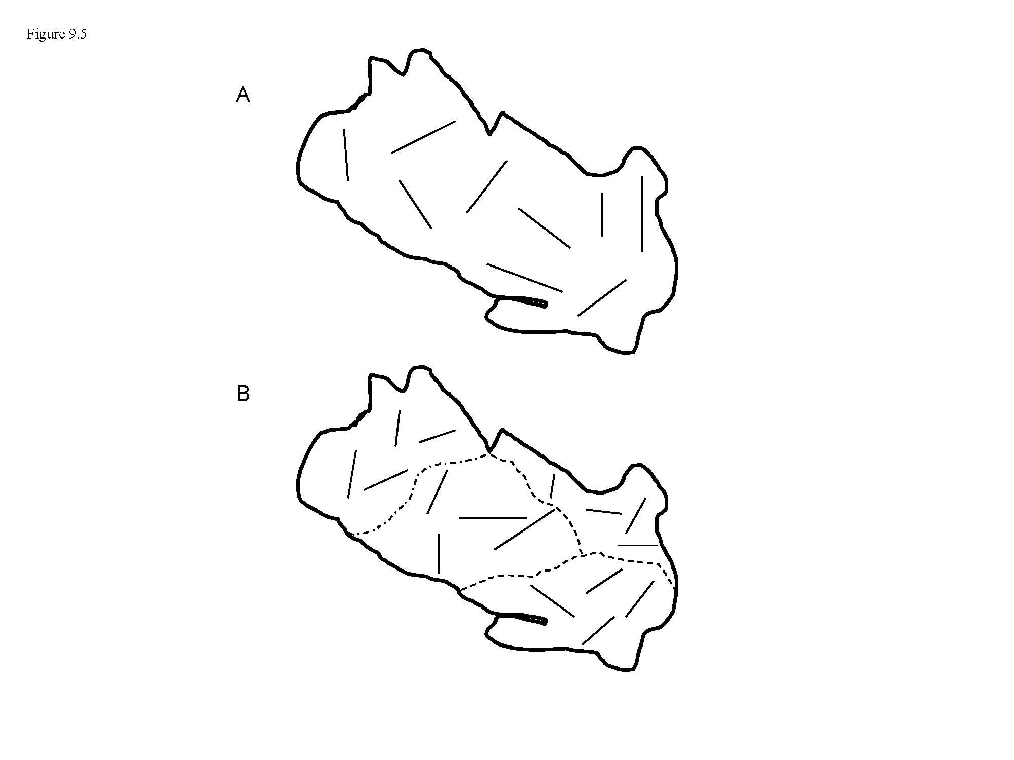
Point transects 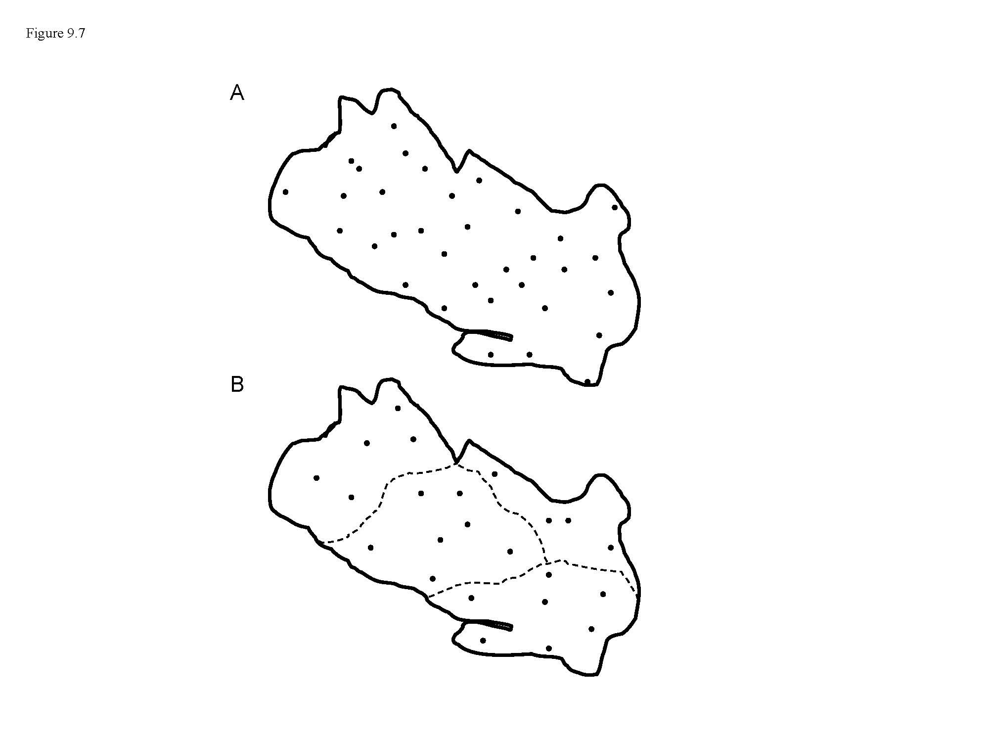
Line transects
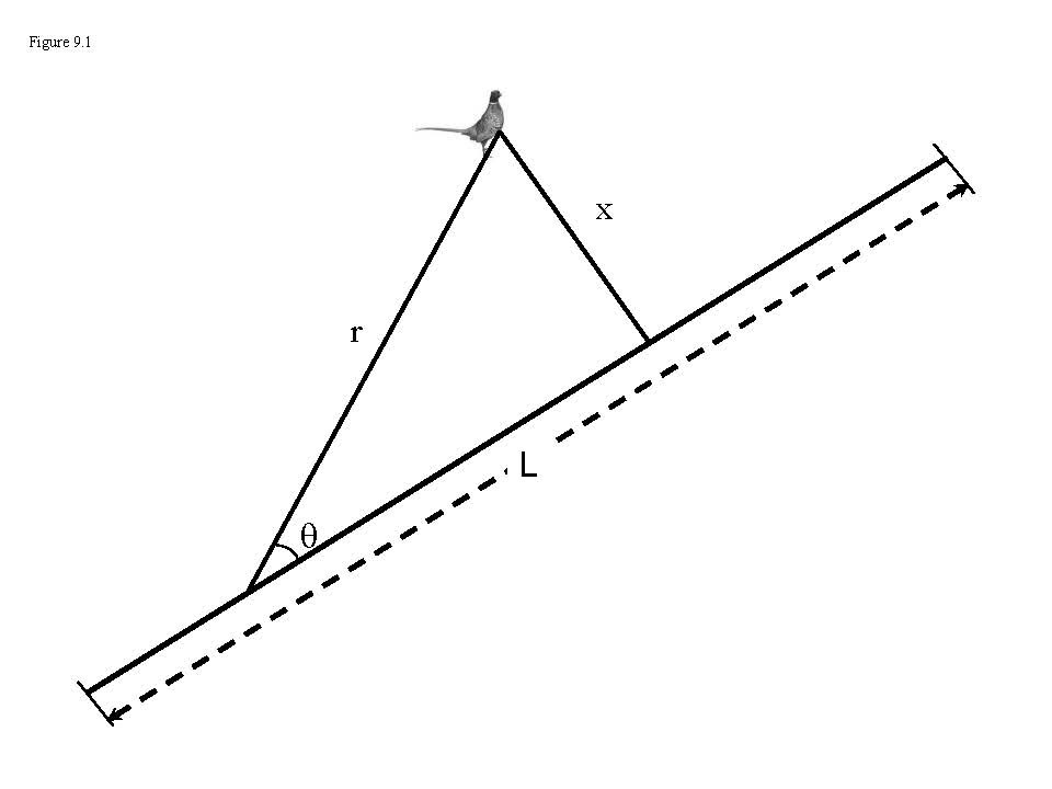
In line transect sampling, it is common to record the radial distance and bearing, rather than the perpendicular distance.
However, the analysis must be conducted on the perpendicular distance data.
Real design
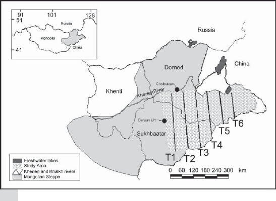
Line transects
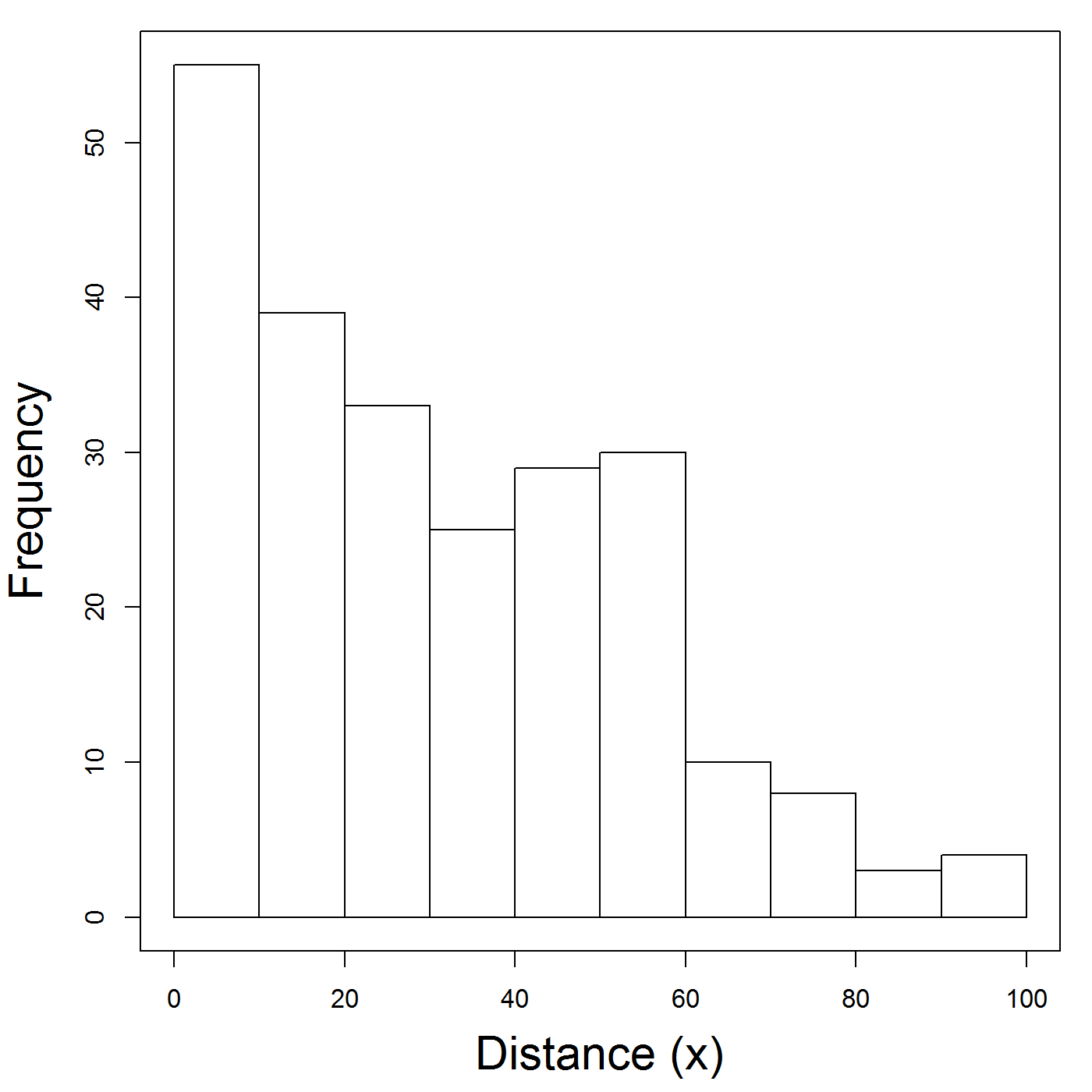
| Animal | Distance (\(x\)) |
|---|---|
| 1 | 4.4 |
| 2 | 25.3 |
| 3 | 41.8 |
| 4 | 3.1 |
| 5 | 78.5 |
| \(\vdots\) | \(\vdots\) |
| \(n\) | 4.4 |
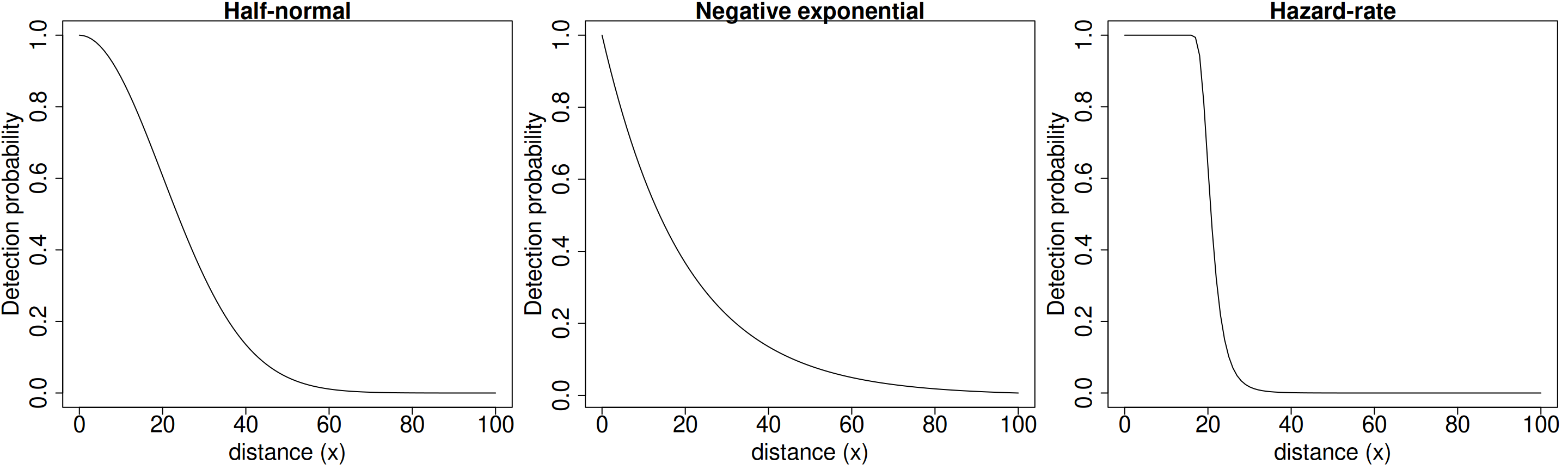
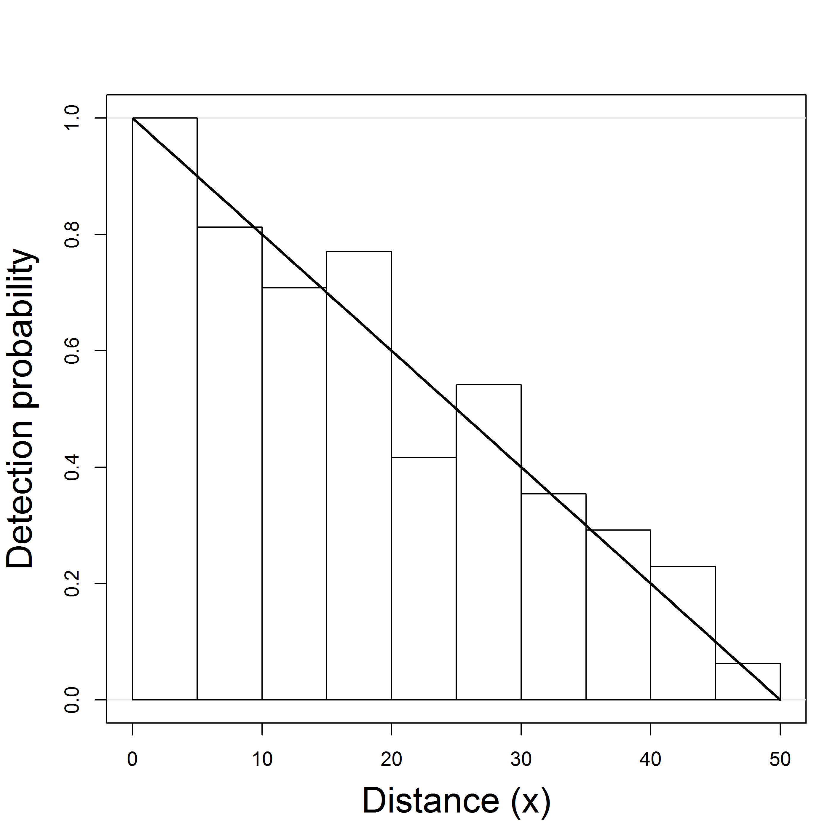
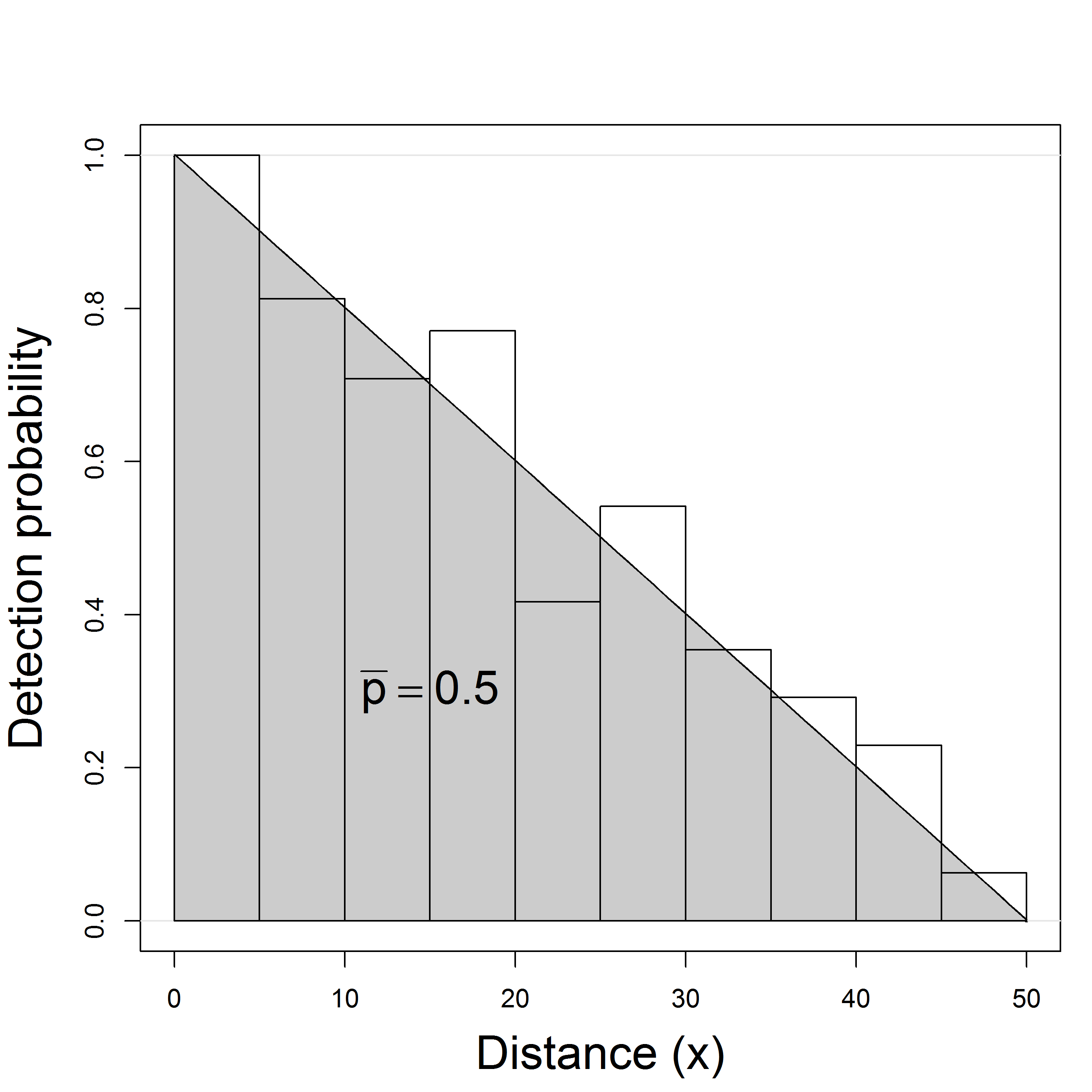
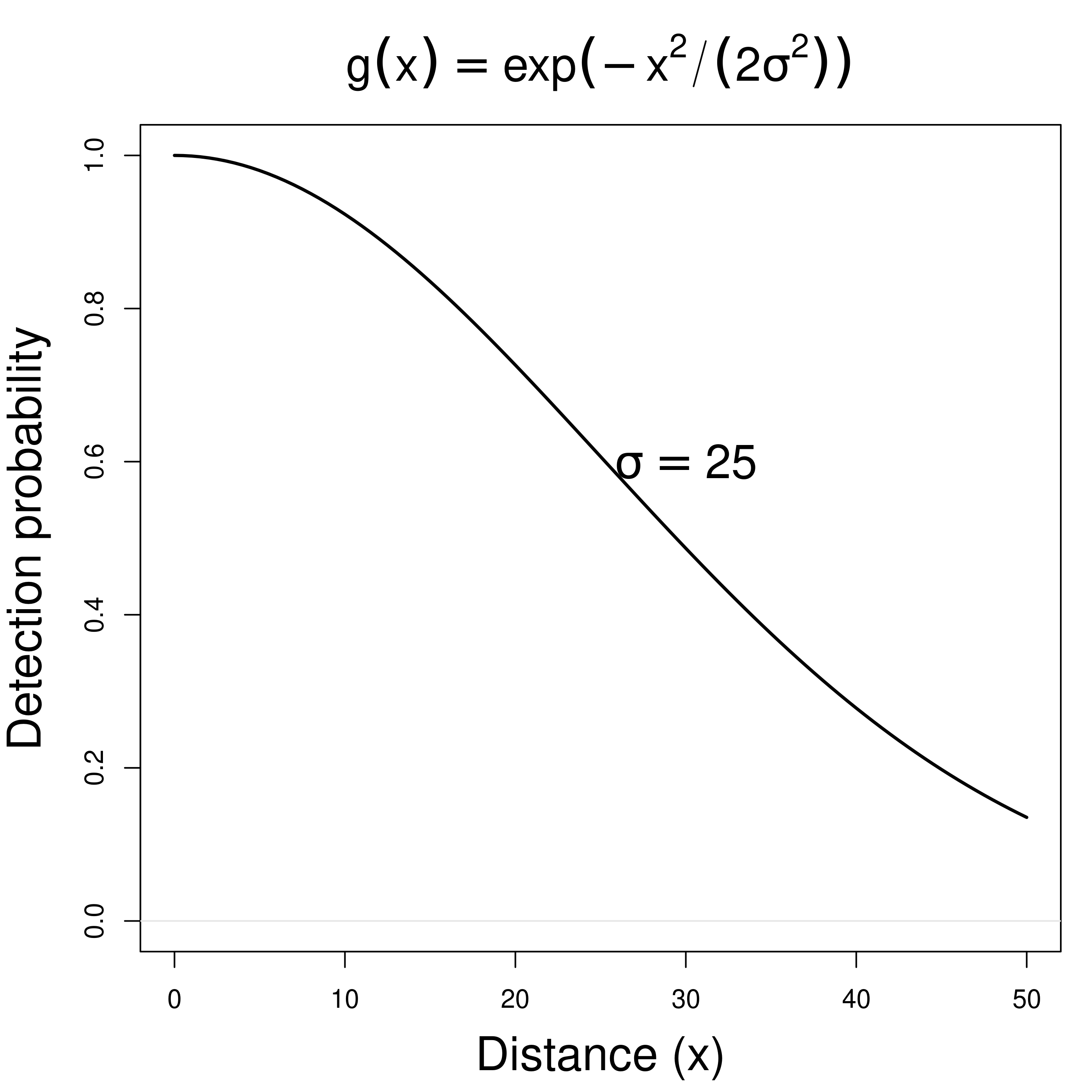
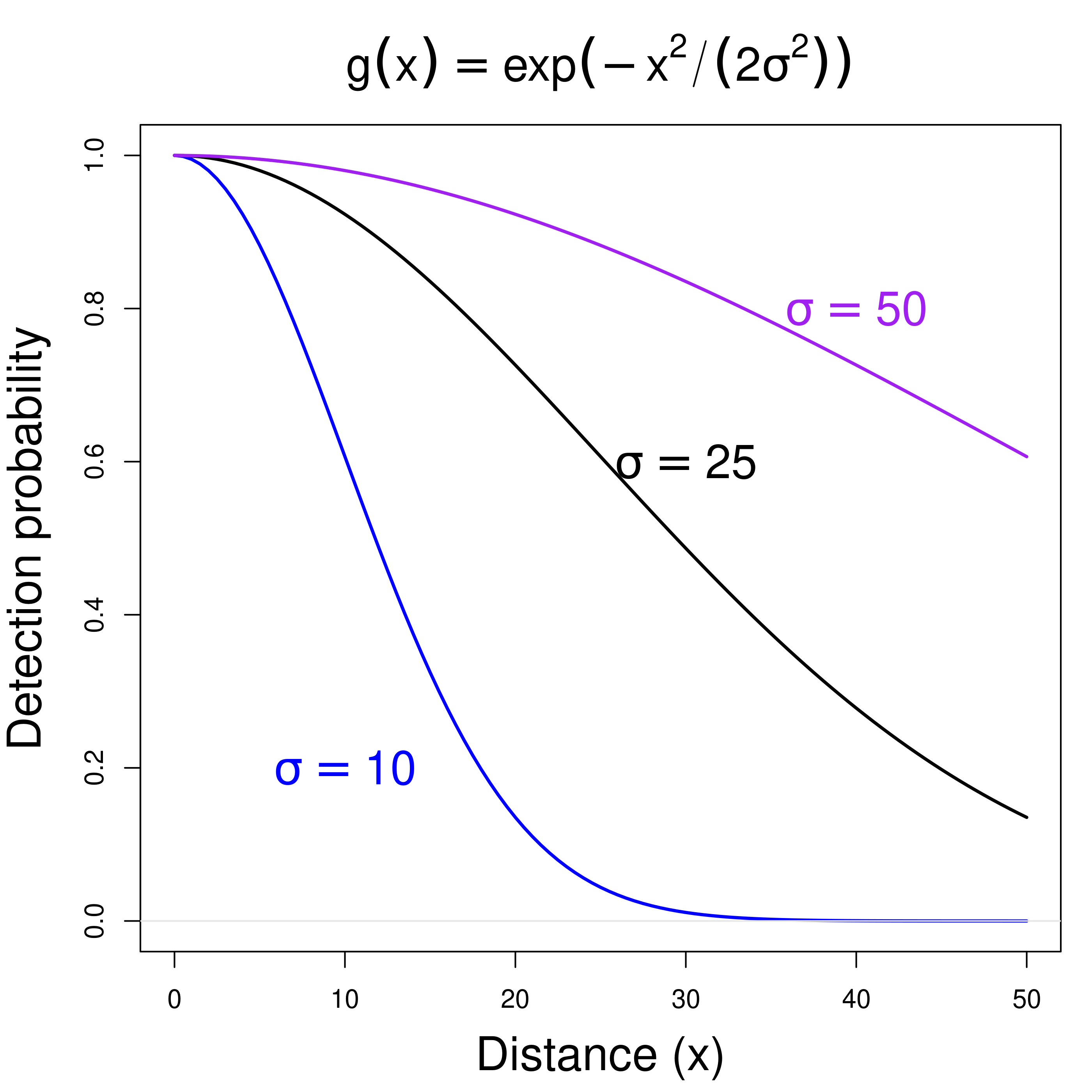
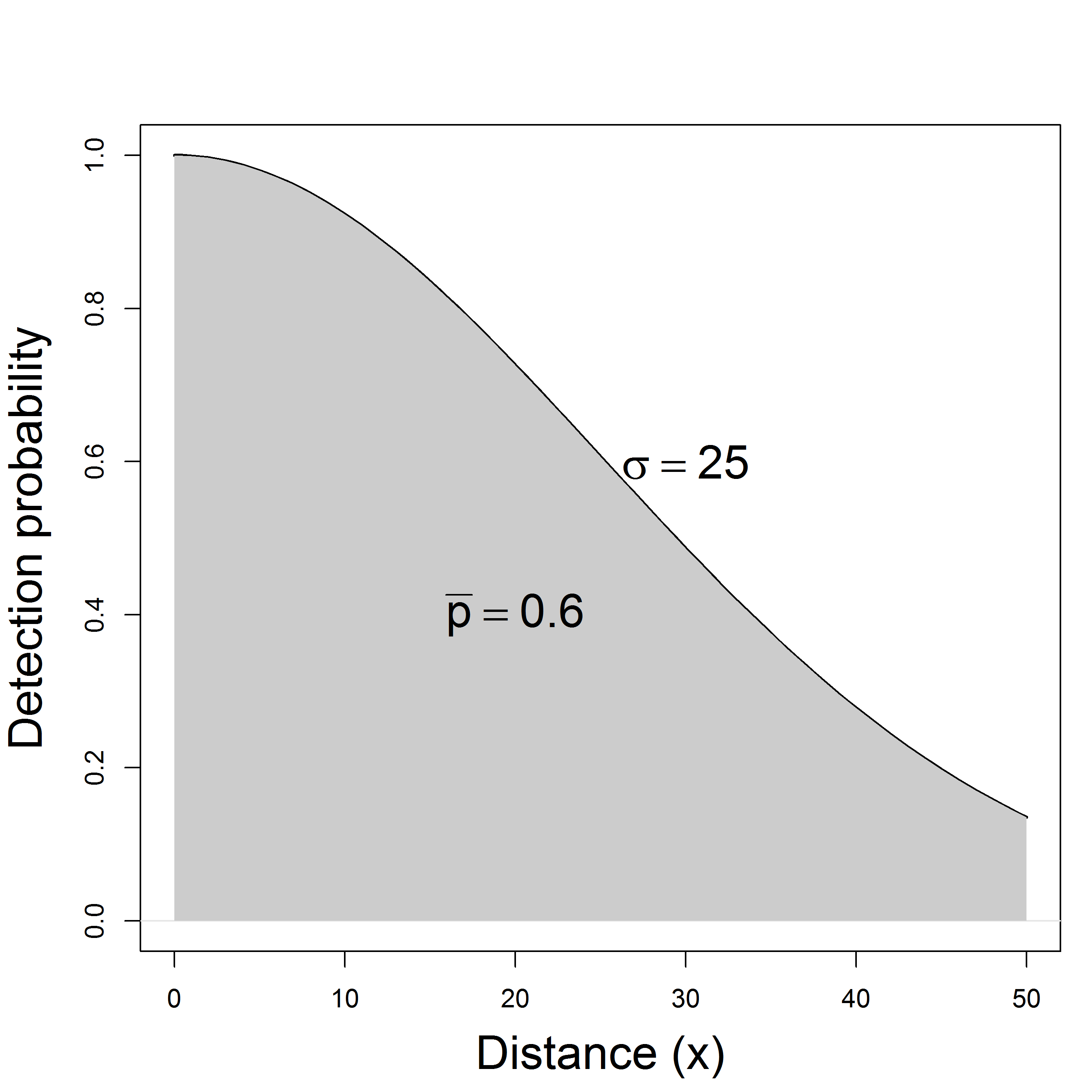
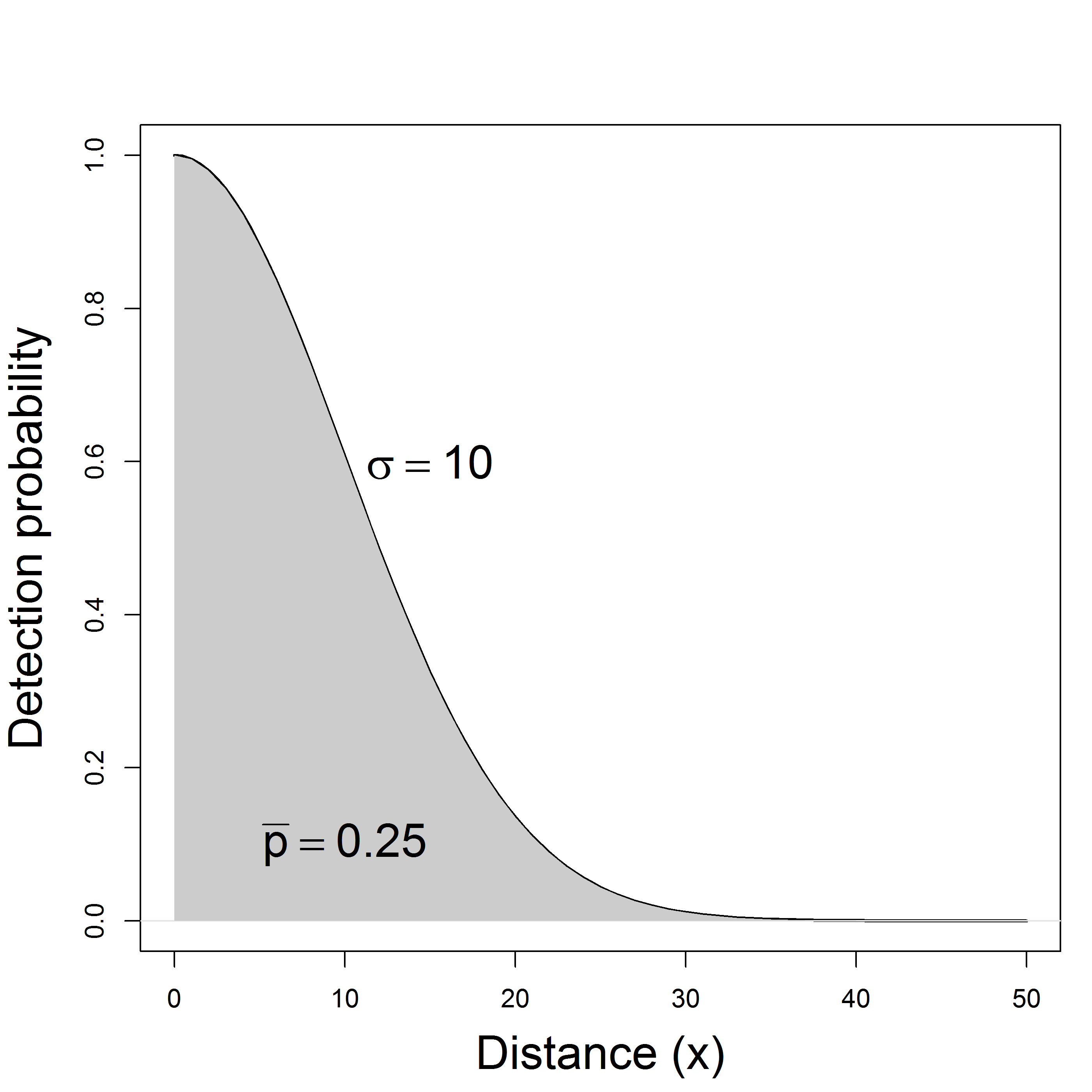
Computing average detection probability
Point transects
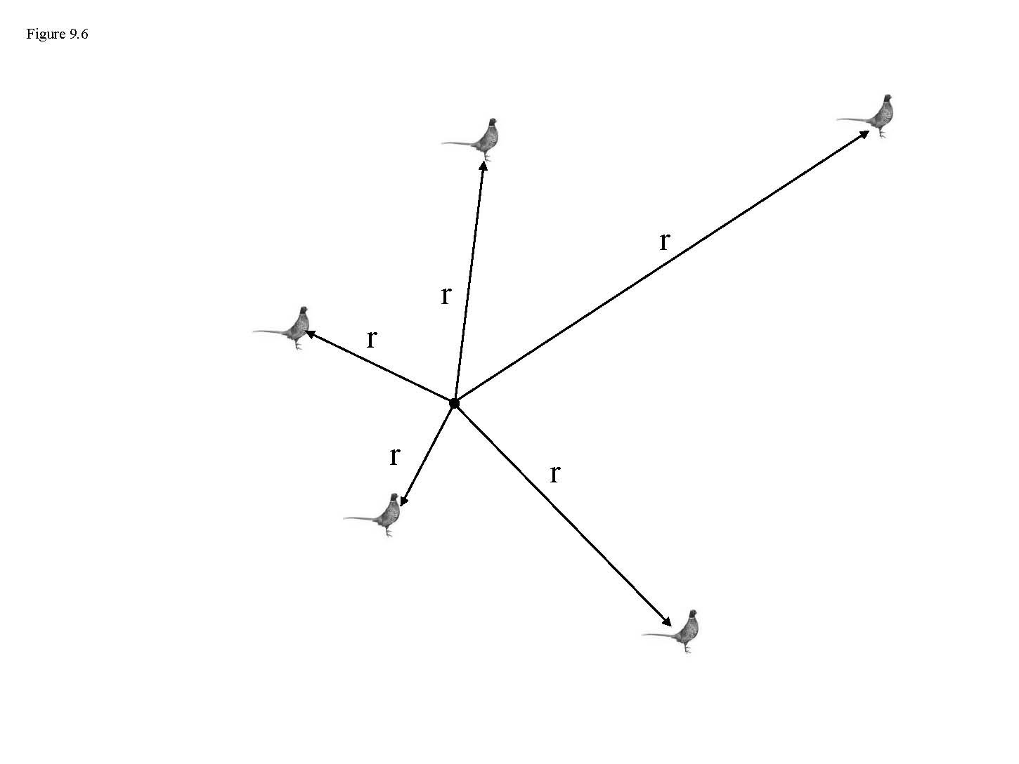
Point Transects
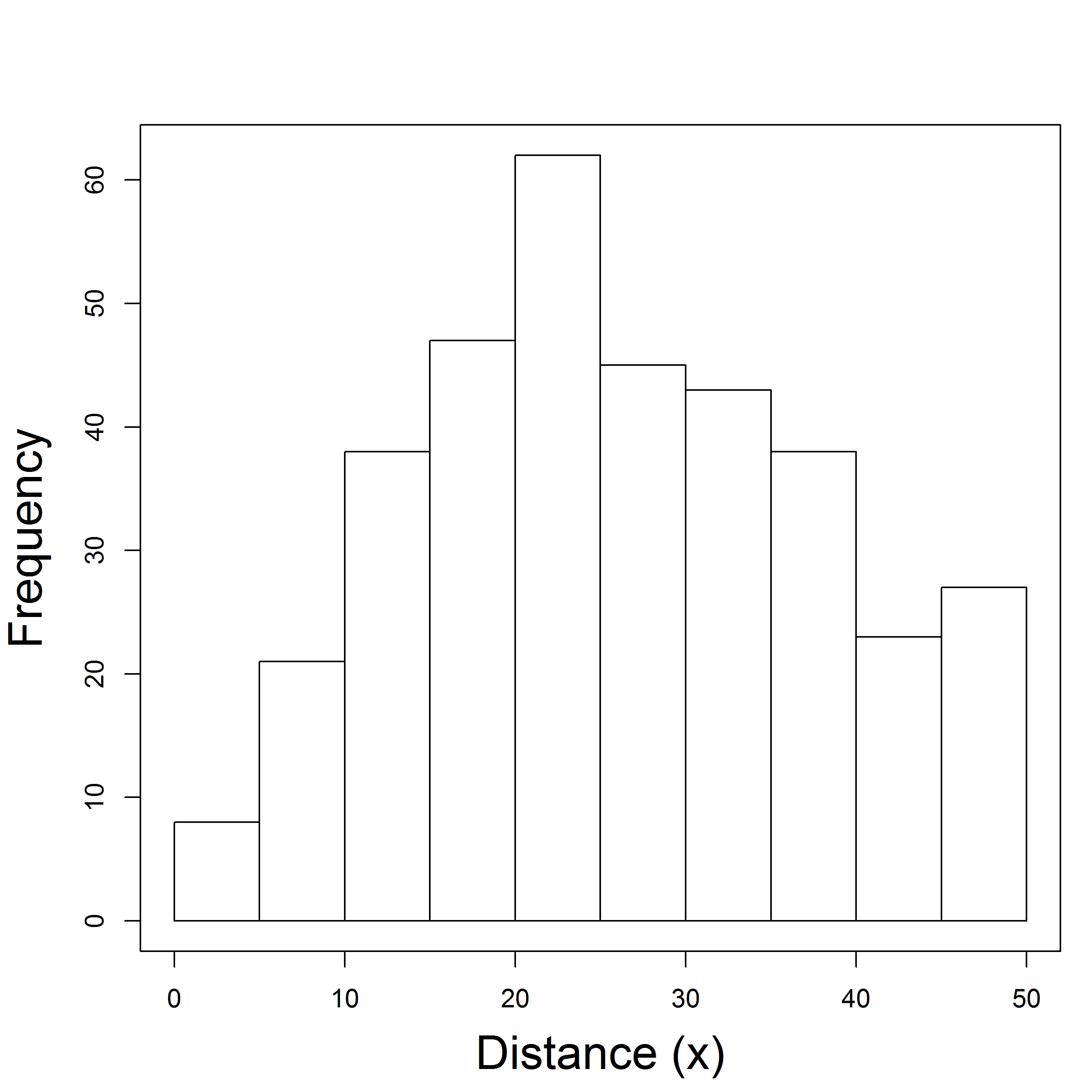
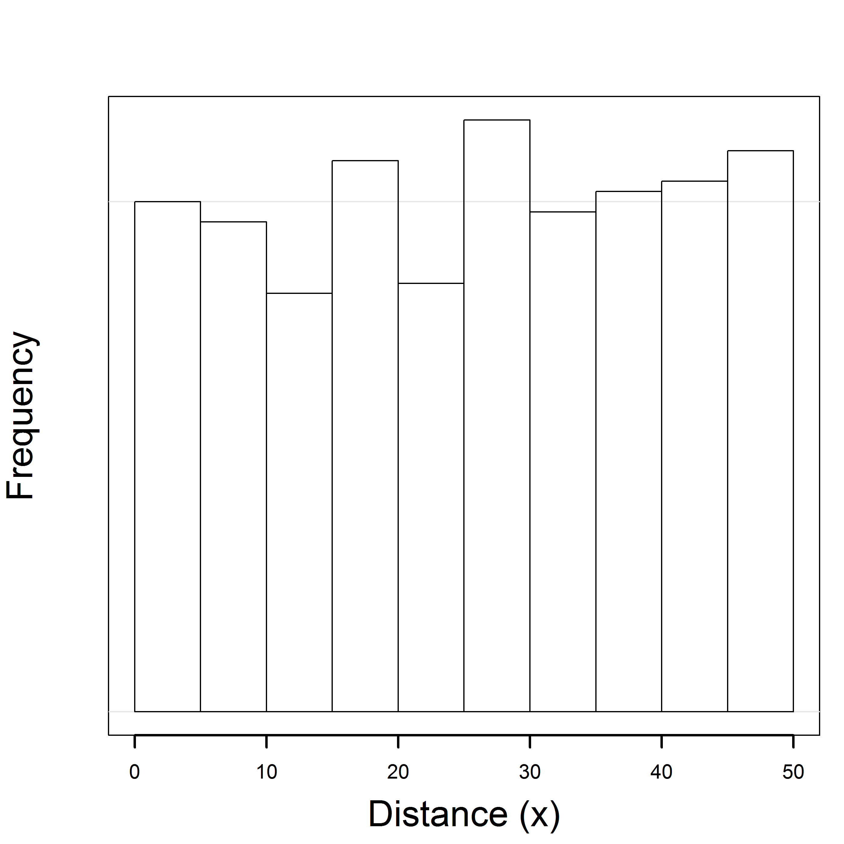
When average detection probability is 1, the histogram of detected distances will increase with area because there are more individuals far from the point.
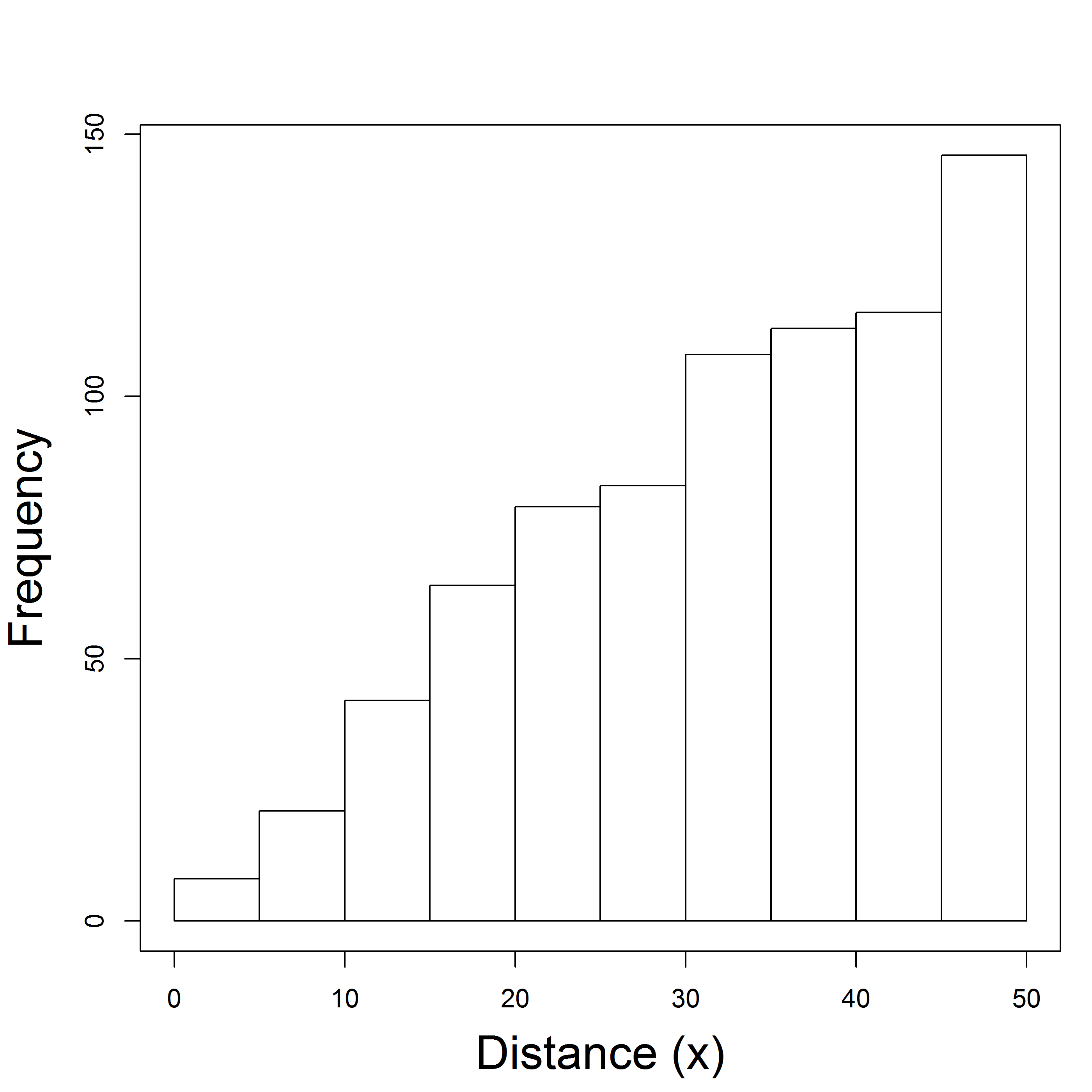
Point Transects
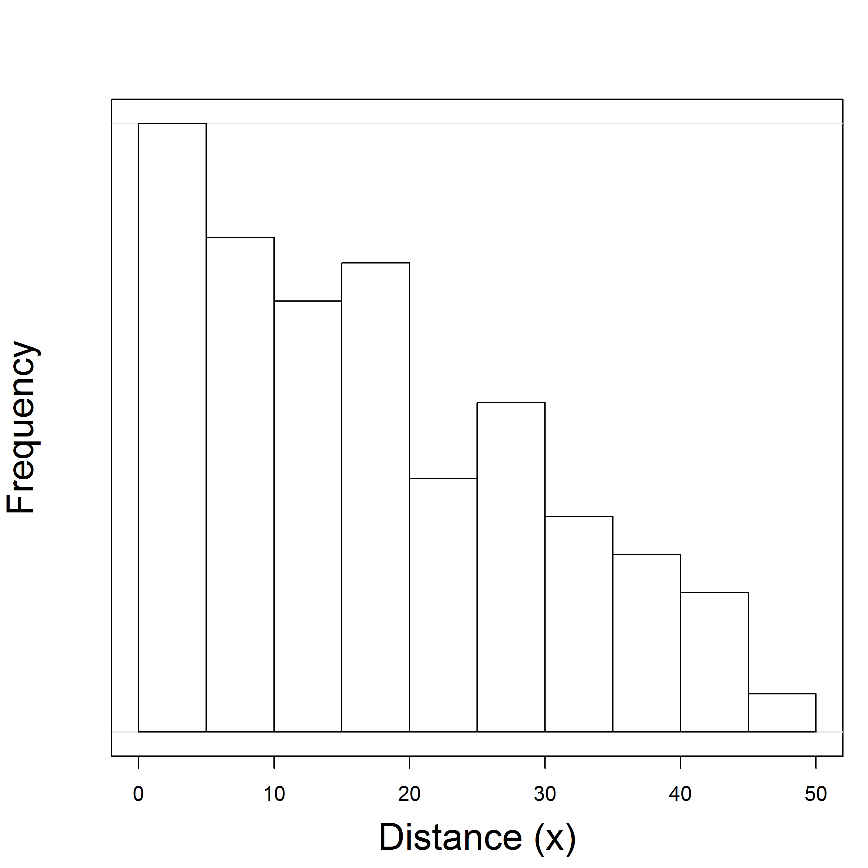
If average detection probability is less than 1, the histogram will increase and then decline.