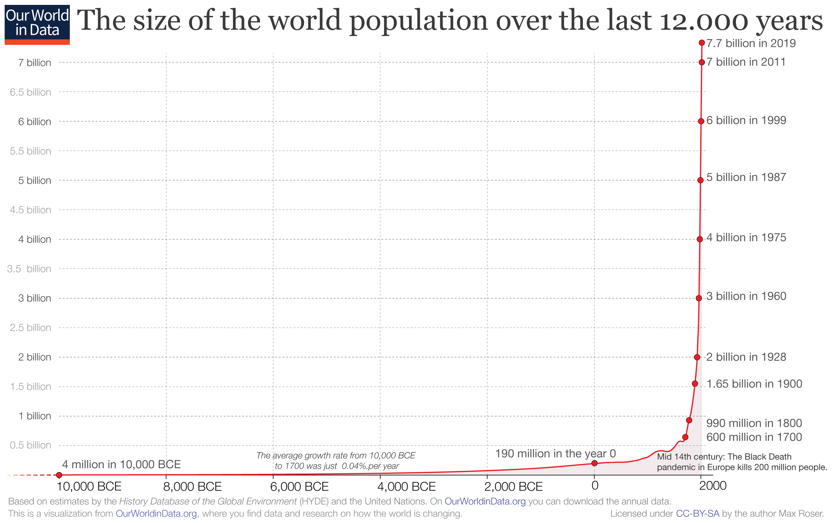
Reverend Thomas Malthus, 1766–1834
Aldo Leopold, Game Management 1946
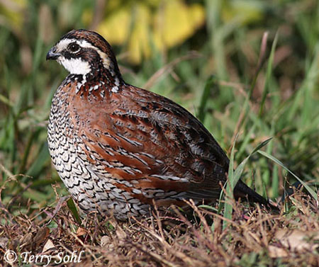
“Every wild species has certain fixed habits which govern the reproductive process, and determine its maximum rate. Thus one pair of quail, if entirely unmolested in an ‘ideal’ environment, would increase at this rate:”
| At End of | Young | Adults | Total |
|---|---|---|---|
| 1st year | 14 | 2 | 16 |
| At End of | Young | Adults | Total |
|---|---|---|---|
| 1st year | 14 | 2 | 16 |
| 2nd year | (16/2)14=112 | 16 | 128 |
| At End of | Young | Adults | Total |
|---|---|---|---|
| 1st year | 14 | 2 | 16 |
| 2nd year | (16/2)14=112 | 16 | 128 |
| 3rd year | (128/2)14=896 | 128 | 1024 |
“The maximum rate of increase is of course never attained in nature. Part of it never takes place, part of it is absorbed by natural enemies, and part of it absorbed by hunters.”
Example
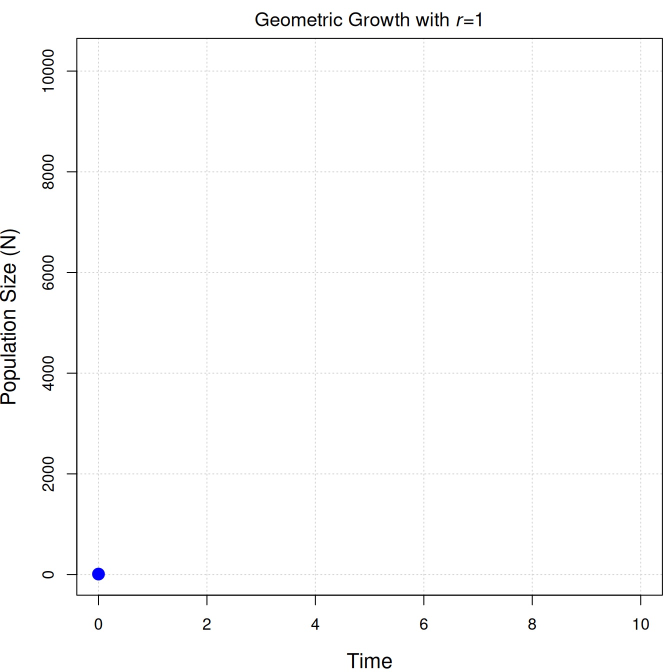
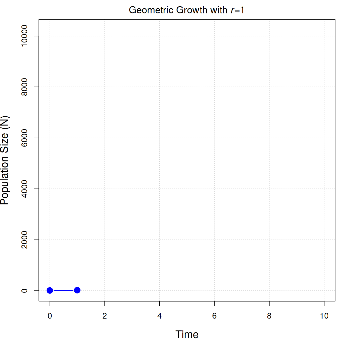
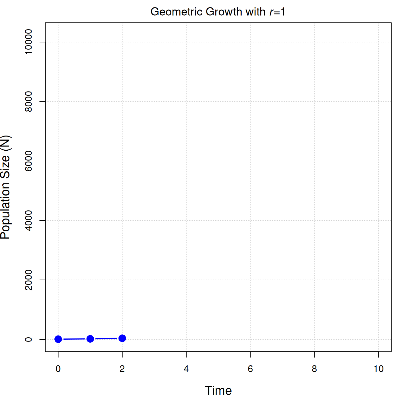
\[N_{t+1} = N_t + N_t r\]
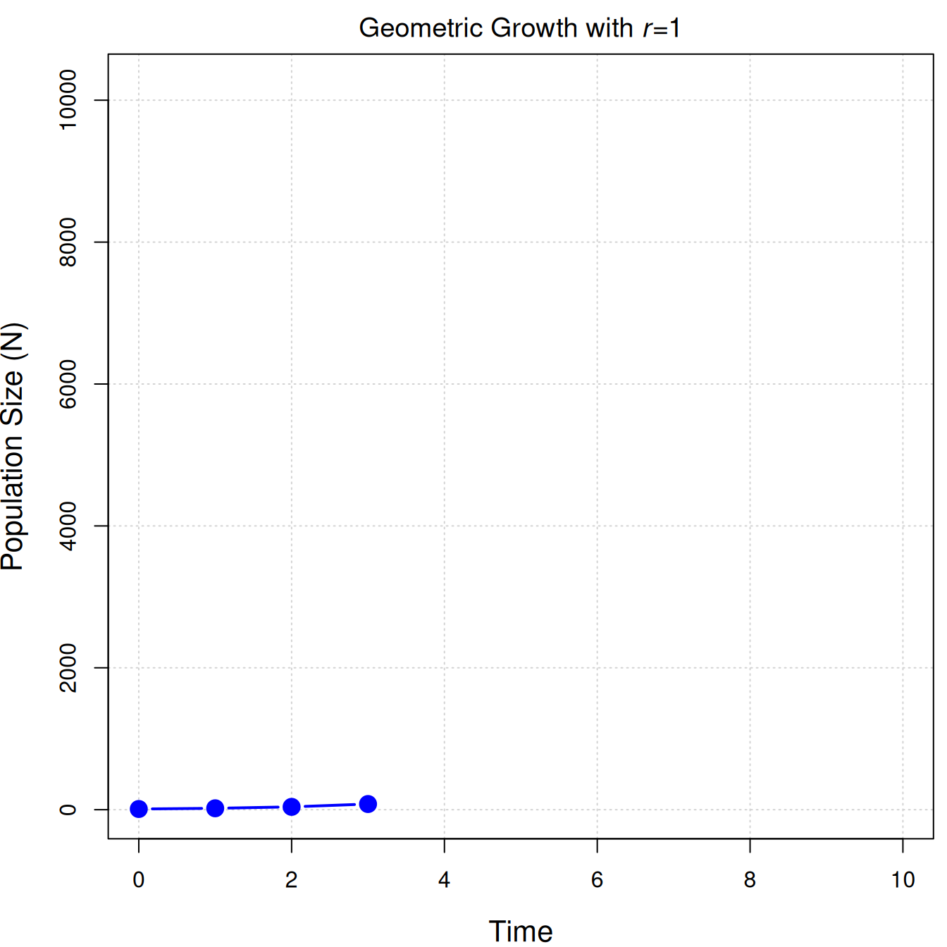
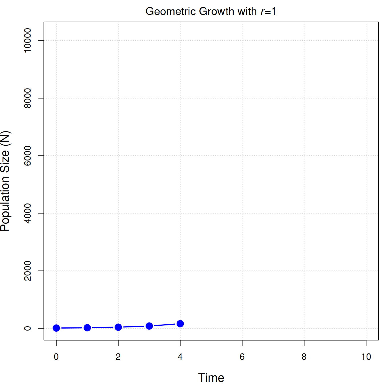
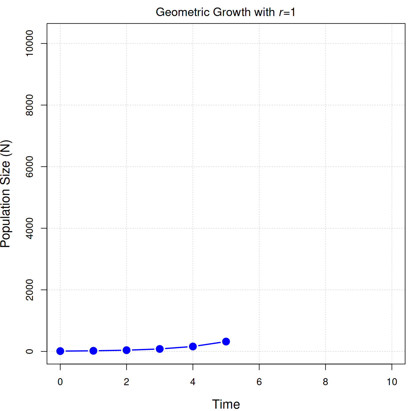
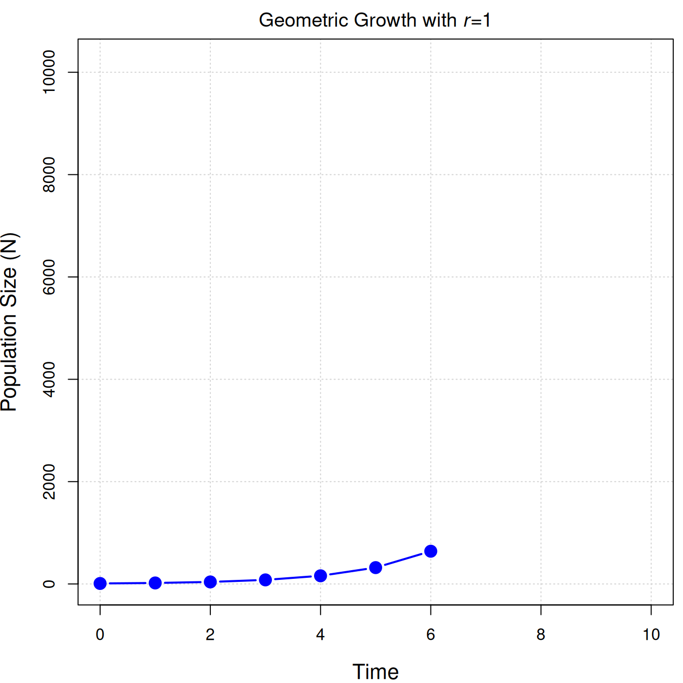
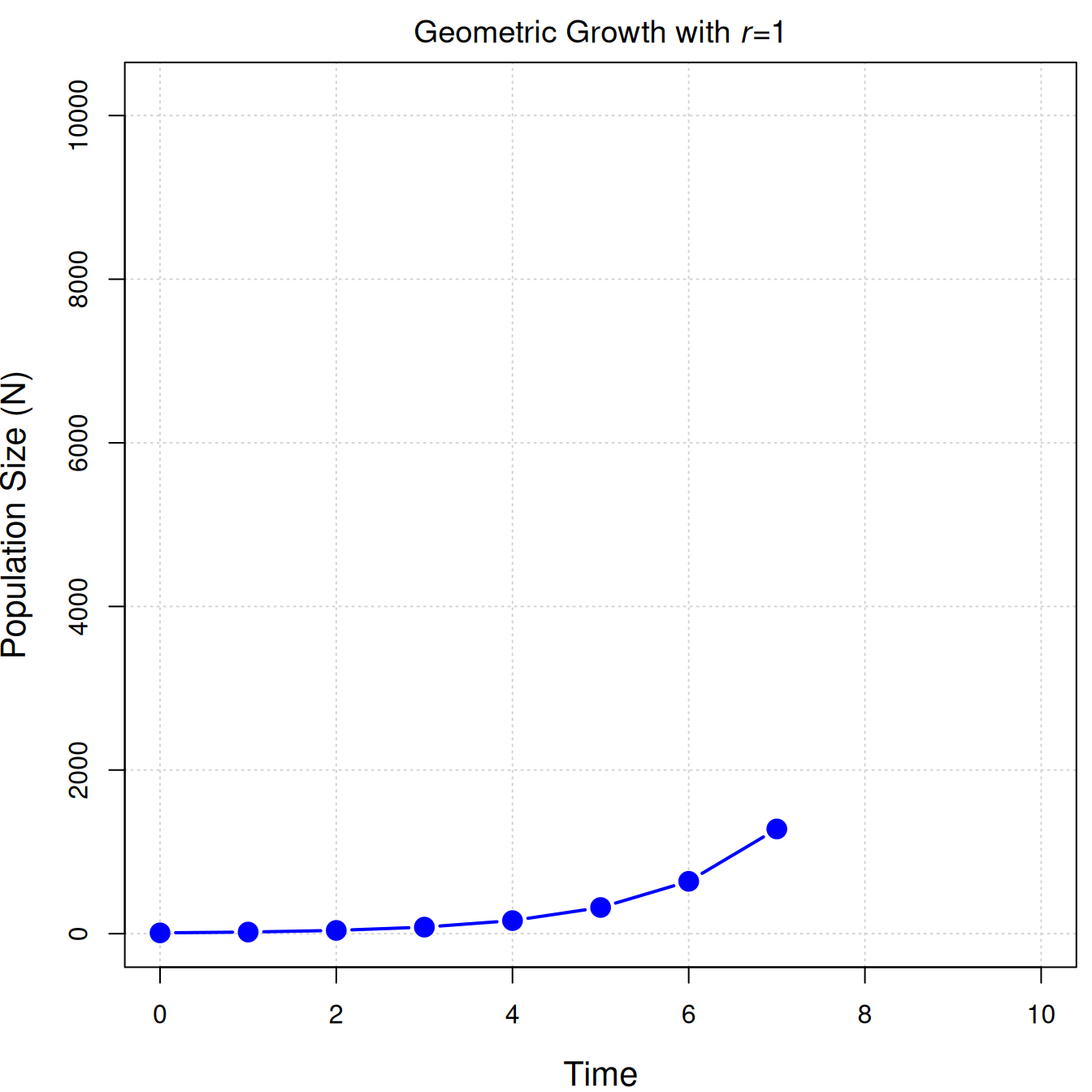
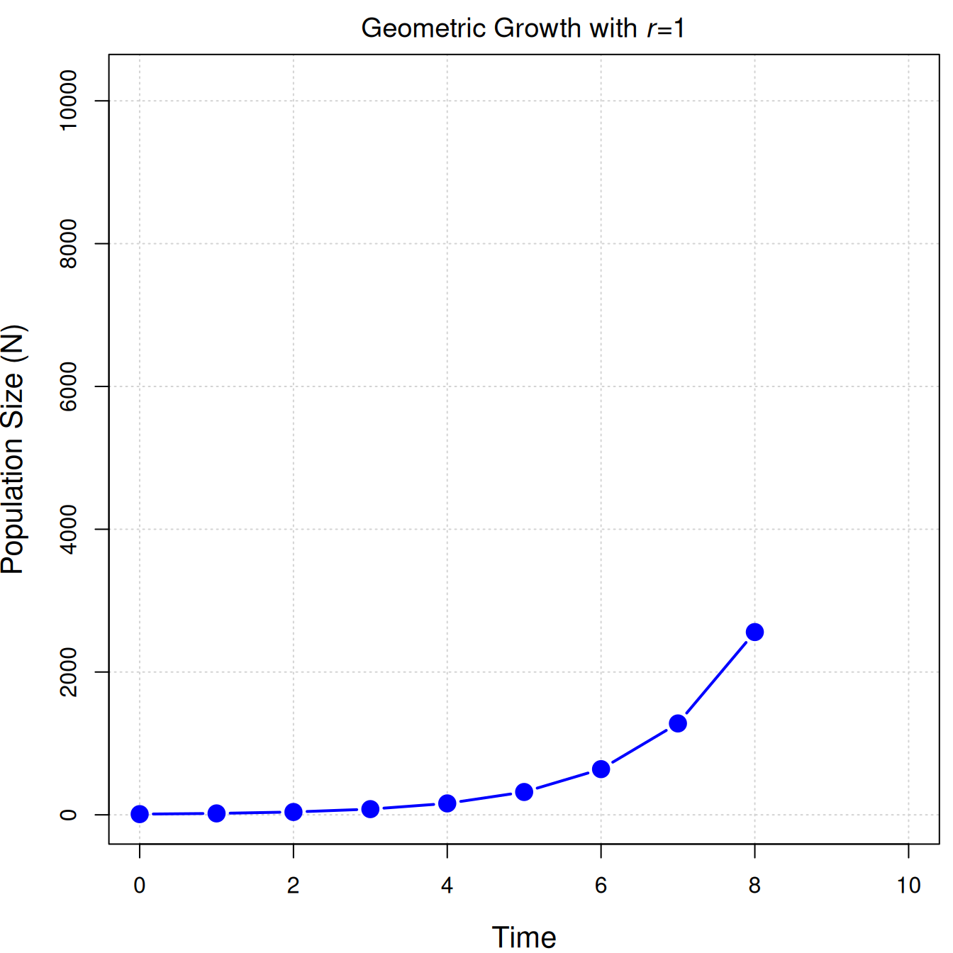
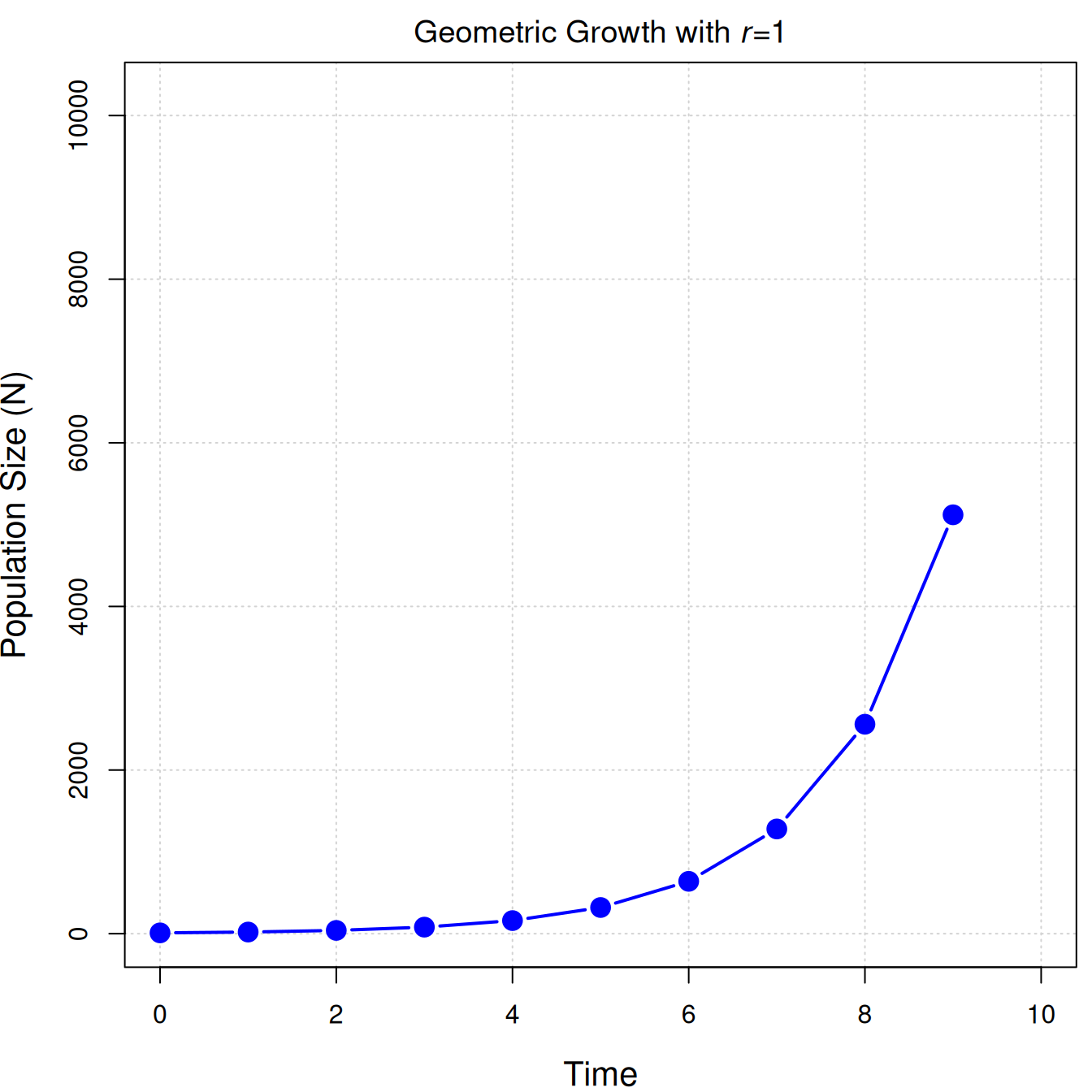
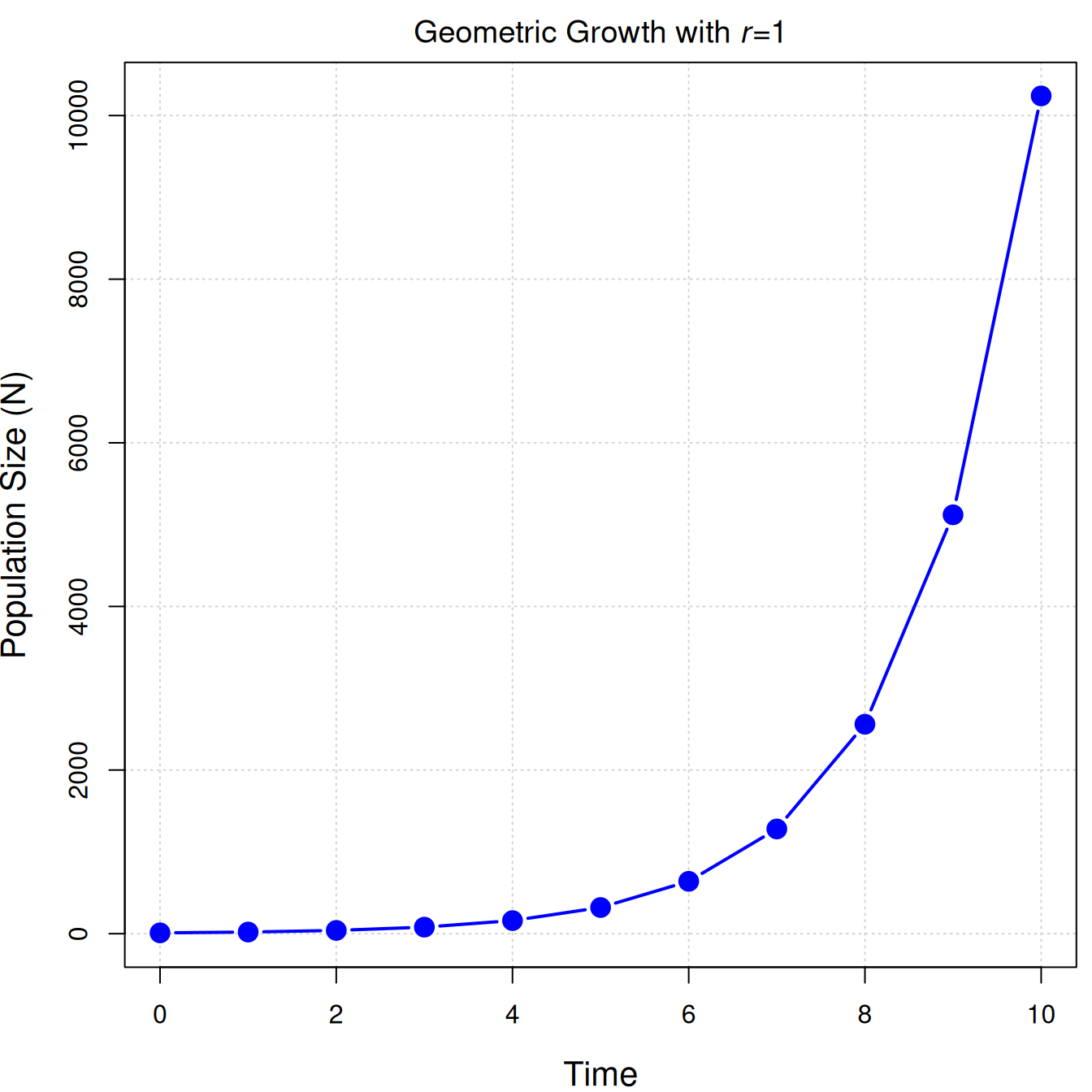
| Time | Population size (\(N\)) |
|---|---|
| 0 | 10 |
| 1 | |
| 2 | |
| 3 | |
| 4 | |
| 5 | |
| 6 | |
| 7 | |
| 8 | |
| 9 | |
| 10 |
| Time | Population size (\(N\)) |
|---|---|
| 0 | 10 |
| 1 | 20 |
| 2 | |
| 3 | |
| 4 | |
| 5 | |
| 6 | |
| 7 | |
| 8 | |
| 9 | |
| 10 |
| Time | Population size (\(N\)) |
|---|---|
| 0 | 10 |
| 1 | 20 |
| 2 | 40 |
| 3 | |
| 4 | |
| 5 | |
| 6 | |
| 7 | |
| 8 | |
| 9 | |
| 10 |
| Time | Population size (\(N\)) |
|---|---|
| 0 | 10 |
| 1 | 20 |
| 2 | 40 |
| 3 | 80 |
| 4 | |
| 5 | |
| 6 | |
| 7 | |
| 8 | |
| 9 | |
| 10 |
| Time | Population size (\(N\)) |
|---|---|
| 0 | 10 |
| 1 | 20 |
| 2 | 40 |
| 3 | 80 |
| 4 | 160 |
| 5 | |
| 6 | |
| 7 | |
| 8 | |
| 9 | |
| 10 |
| Time | Population size (\(N\)) |
|---|---|
| 0 | 10 |
| 1 | 20 |
| 2 | 40 |
| 3 | 80 |
| 4 | 160 |
| 5 | 320 |
| 6 | |
| 7 | |
| 8 | |
| 9 | |
| 10 |
| Time | Population size (\(N\)) |
|---|---|
| 0 | 10 |
| 1 | 20 |
| 2 | 40 |
| 3 | 80 |
| 4 | 160 |
| 5 | 320 |
| 6 | 640 |
| 7 | |
| 8 | |
| 9 | |
| 10 |
| Time | Population size (\(N\)) |
|---|---|
| 0 | 10 |
| 1 | 20 |
| 2 | 40 |
| 3 | 80 |
| 4 | 160 |
| 5 | 320 |
| 6 | 640 |
| 7 | 1280 |
| 8 | |
| 9 | |
| 10 |
| Time | Population size (\(N\)) |
|---|---|
| 0 | 10 |
| 1 | 20 |
| 2 | 40 |
| 3 | 80 |
| 4 | 160 |
| 5 | 320 |
| 6 | 640 |
| 7 | 1280 |
| 8 | 2560 |
| 9 | |
| 10 |
| Time | Population size (\(N\)) |
|---|---|
| 0 | 10 |
| 1 | 20 |
| 2 | 40 |
| 3 | 80 |
| 4 | 160 |
| 5 | 320 |
| 6 | 640 |
| 7 | 1280 |
| 8 | 2560 |
| 9 | 5120 |
| 10 |
| Time | Population size (\(N\)) |
|---|---|
| 0 | 10 |
| 1 | 20 |
| 2 | 40 |
| 3 | 80 |
| 4 | 160 |
| 5 | 320 |
| 6 | 640 |
| 7 | 1280 |
| 8 | 2560 |
| 9 | 5120 |
| 10 | 10240 |
Three Possible Outcomes
\[N_{t+1} = N_t + N_t r\]
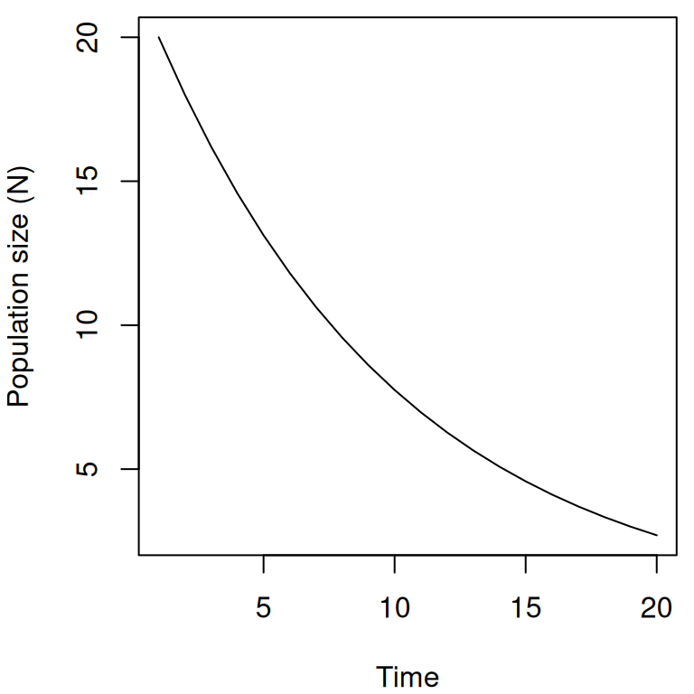
\(-1 \leq r < 0\)
population goes extinct
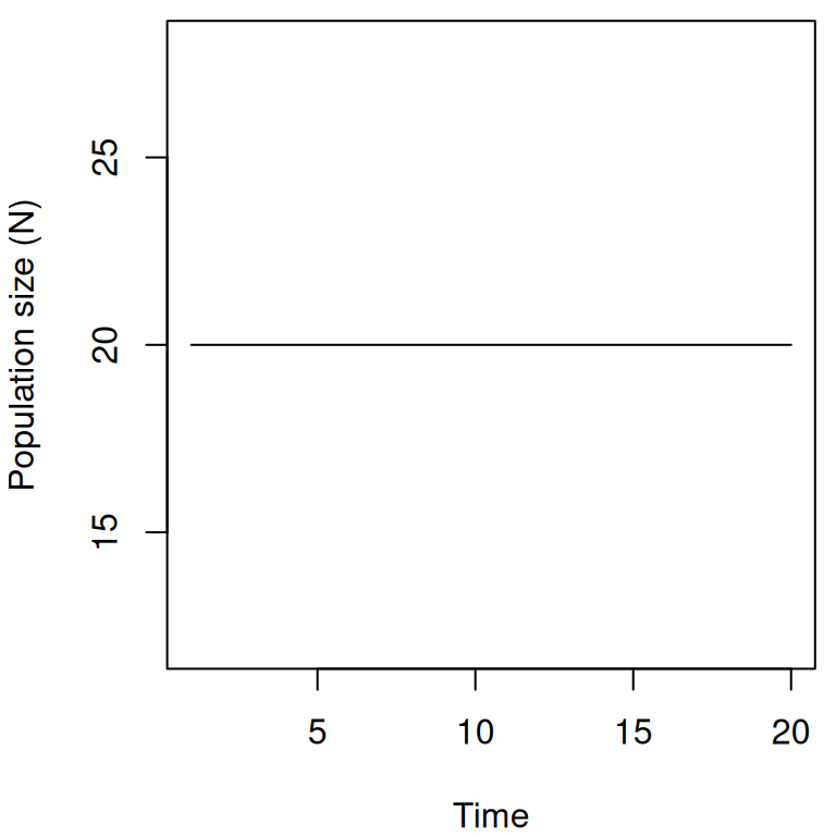
\(r = 0\)
population is at equilibrium
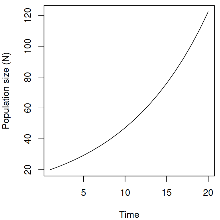
\(r > 0\)
population grows to \(\infty\)
Can We Apply The Model To Real Data?
All models are wrong, but some are useful. (George Box)
Is exponential growth a useful model?
Possibly for describing some populations during short time periods.
And as foundation for more realistic models.
Looking Ahead
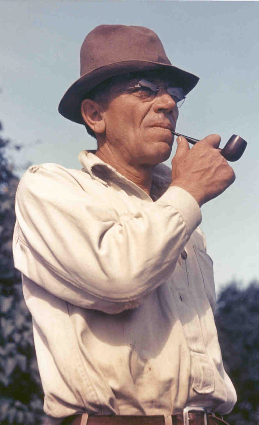
Is the human population exhibiting exponential growth?