Occupancy Estimation and Modeling
Motivation
Occupancy models were developed to estimate metapopulation parameters when detection probability (\(p\)) is \(<1\).
\[ \psi_{i,t+1} = O_{i,t}(1-\varepsilon) + (1-O_{i,t})\gamma \\ O_{i,t+1} \sim \mbox{Bernoulli}(\psi_{i,t+1}) \]
Metapopulation parameters:
- \(\psi\) – Probability that a site is occupied
- \(\gamma\) – Probability that an unoccupied site becomes colonized
- \(\varepsilon\) – Probability that an occupied site goes extinct
- \(p\) – Probability of detecting at least one individual at a site that is occupied (on a single sampling occasion)
Detection probability
If \(p<1\), we might incorrectly conclude that a site is unoccupied if we don’t detect any individuals
Consequences:
- We will underestimate the state variable: The proportion of sites occupied
- We might make incorrect conclusions about habitat relationships
Single-season models
Scenario
- No interest in colonization or extinction events
- Instead, we directly estimate \(\psi\) during one season
- Useful for assessing snapshot of habitat relationships or for modeling a species’ distribution
- We assume population closure: A site’s occupancy state does not change during the survey period (season)
- Definitions of site and season are very important
How many potholes are occupied by mallards?
Single-season model
Model for the occurrence state \[ O_{i} \sim \mbox{Bernoulli}(\psi) \]
Model for the data \[ y_{ij} \sim \mbox{Bernoulli}(O_i \times p) \]
Design
To estimate \(\psi\) and \(p\), we should use a good study design:
- We need multiple sites
- Sites should be randomly selected
- We must have multiple sampling occasions at (a subset of) the sites
Data yij – low detection probability
| Occasion 1 | Occasion 2 | Occasion 3 | |
|---|---|---|---|
| Site 1 | 0 | 0 | 1 |
| Site 2 | 0 | 0 | 0 |
| Site 3 | 0 | 0 | 0 |
| Site 4 | 1 | 0 | 0 |
| Site 5 | 0 | 0 | 0 |
| Site 6 | 1 | 0 | 1 |
| Site 7 | 1 | 0 | 0 |
| Site 8 | 0 | 0 | 0 |
| Site 9 | 0 | 1 | 0 |
| Site 10 | 0 | 0 | 0 |
Data yij – high detection probability
| Occasion 1 | Occasion 2 | Occasion 3 | |
|---|---|---|---|
| Site 1 | 1 | 1 | 1 |
| Site 2 | 0 | 0 | 0 |
| Site 3 | 0 | 0 | 0 |
| Site 4 | 1 | 1 | 1 |
| Site 5 | 0 | 0 | 0 |
| Site 6 | 1 | 0 | 1 |
| Site 7 | 1 | 1 | 1 |
| Site 8 | 0 | 0 | 0 |
| Site 9 | 0 | 1 | 1 |
| Site 10 | 0 | 0 | 0 |
How do we estimate \(\psi\) and \(p\)?
Maximum likelihood
- This method tries to find the most “likely” values of \(\psi\) and \(p\), given the data
- It can also be used to estimate standard errors (SEs) and confidence intervals (CIs)
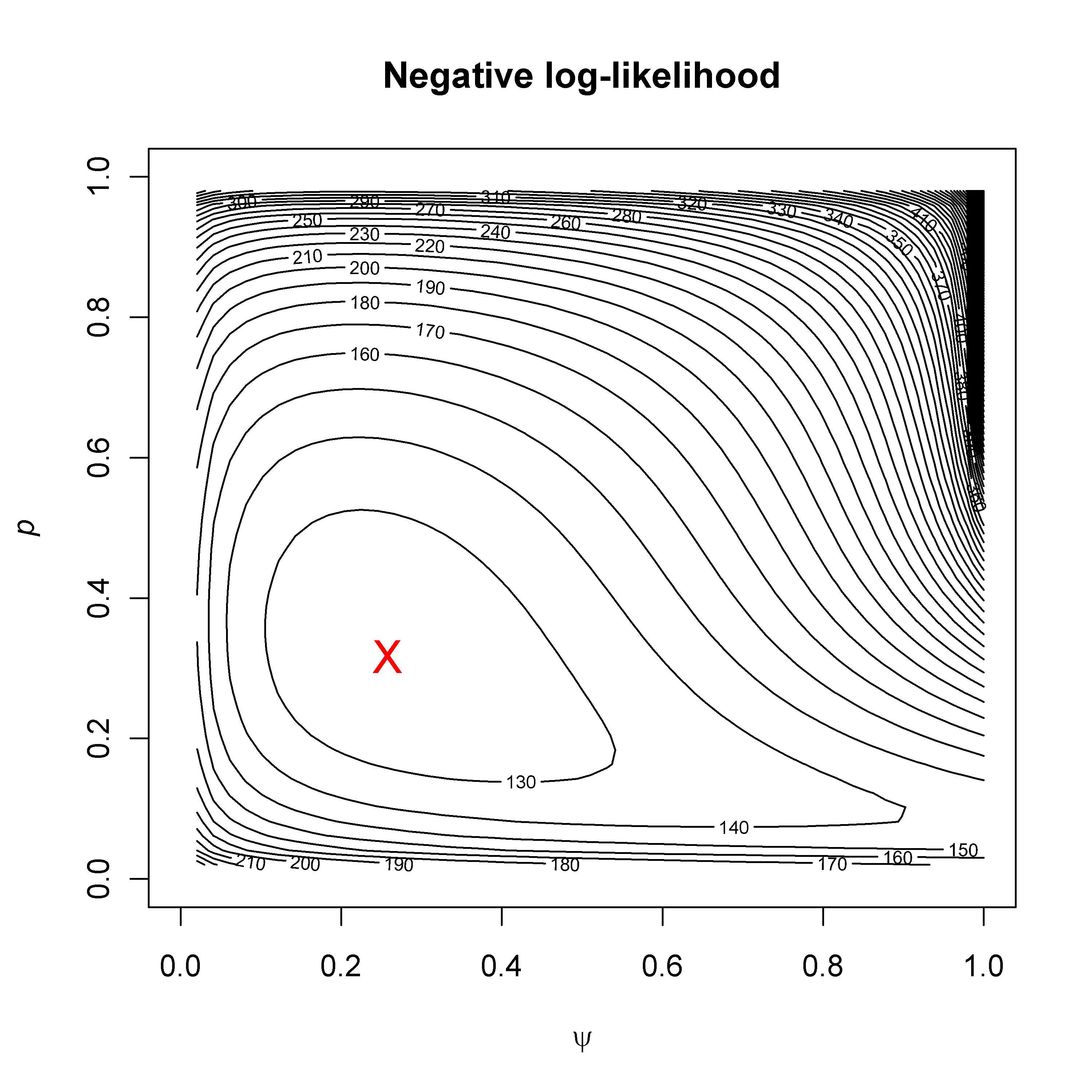
Software: Program PRESENCE, Program MARK, R package unmarked
Estimates
| Occasion 1 | Occasion 2 | Occasion 3 | |
|---|---|---|---|
| Site 1 | 0 | 0 | 1 |
| Site 2 | 0 | 0 | 0 |
| Site 3 | 0 | 0 | 0 |
| Site 4 | 1 | 1 | 0 |
| Site 5 | 0 | 0 | 0 |
| Site 6 | 1 | 1 | 1 |
| Site 7 | 1 | 0 | 0 |
| Site 8 | 0 | 0 | 0 |
| Site 9 | 0 | 1 | 0 |
| Site 10 | 0 | 0 | 0 |
Naive occupancy = 5/10 = 0.50
Estimated occupancy = \(\hat{\psi} = 0.61 \pm 0.22\)
Estimated detection = \(\hat{p} = 0.44 \pm 0.16\)
Overall detection probability
If you sample a site \(K\) times, how do you calculate overall detection probability (\(\bar{p}\))?
\[ \bar{p} = 1 - (1-p)^K \]
\(\bar{p}\) is detection probability after \(K\) sampling occasions
\(p\) is detection probability on a single occasion
\(K\) is the number of sampling occasions (e.g., visits to a site)
Assumptions
- Population closure: Occurrence state does not change during sampling
- Occurrence probability is the same for all sites, unless we account for covariates
- Detection probability is the same for all sites and sampling occasions, unless we account for covariates
- Statistical independence
Covariates
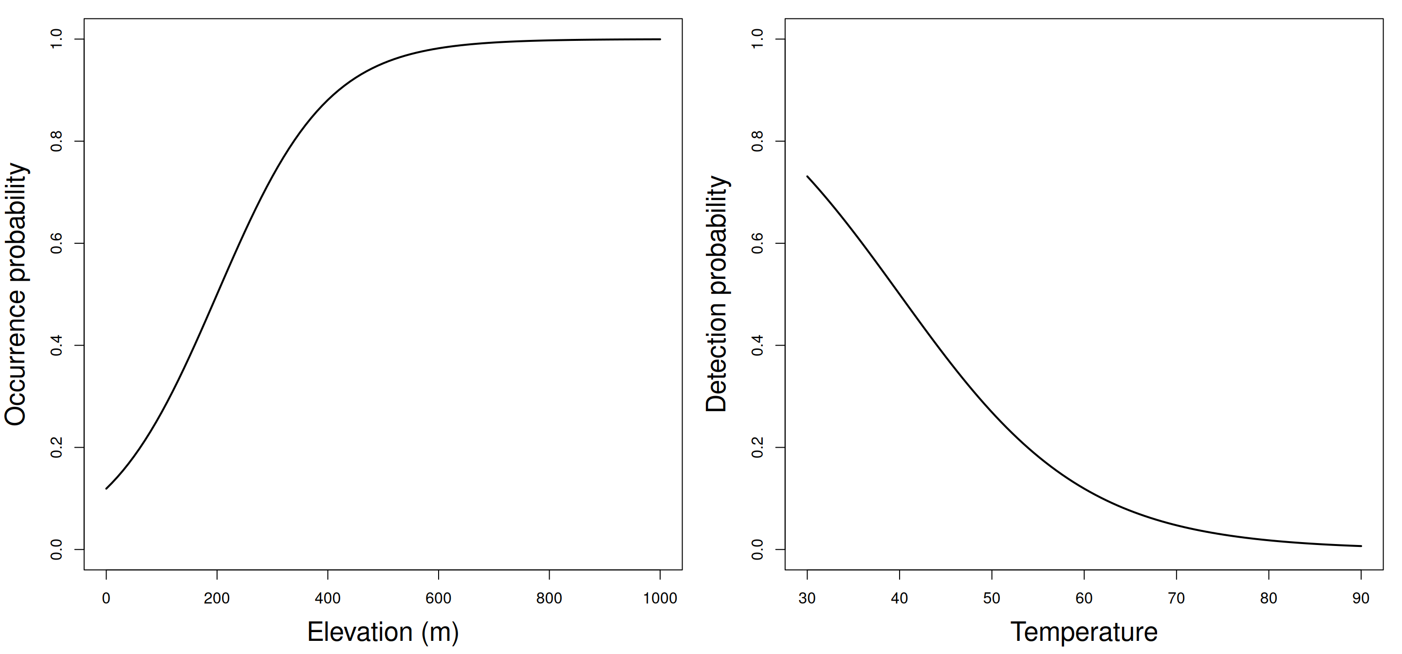
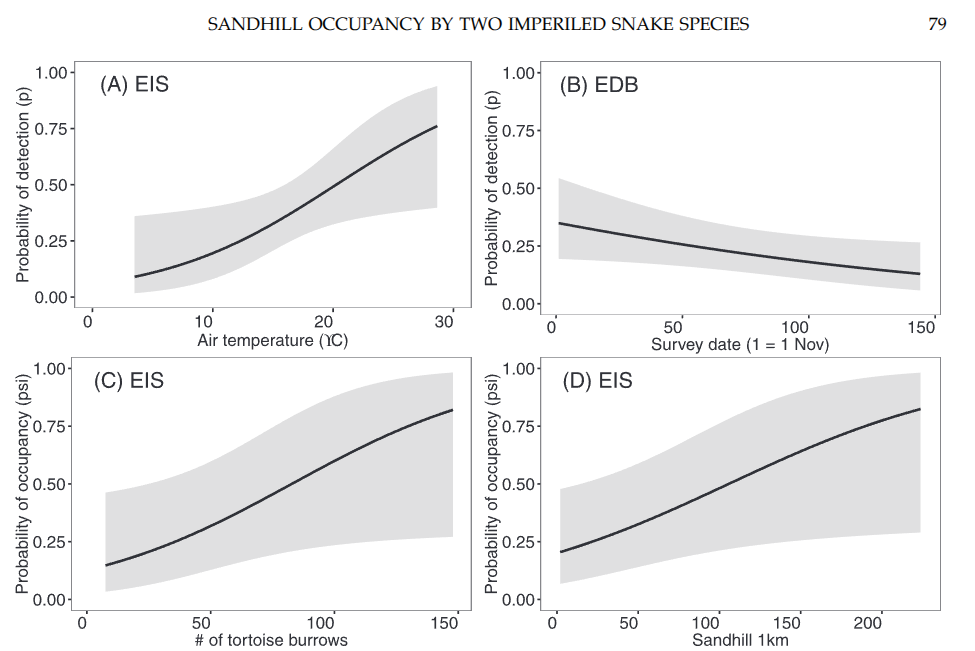
The value of \(\psi\) or \(p\) may depend on other variables, e.g. habitat, weather, observer abilities.
Covariate effects can be accounted for by treating detection probability as a function.
A common choice is the logit-linear model: \[ \mbox{logit}(\psi_i) = \beta_0 + \beta_1\mbox{ELEV}_i \]
Covariates
Example
Example
Bauder et al. 2017
Multi-season models
Multi-season models
With more than 1 season, we can estimate all the parameters of our metapopulation model, plus detection probability \(p\)
\[ \psi_{i,t+1} = O_{i,t}(1-\varepsilon) + (1-O_{i,t})\gamma \\ O_{i,t+1} \sim \mbox{Bernoulli}(\psi_{i,t+1}) \\ y_{i,j,t} \sim \mathrm{Bernoulli}(O_{i,t} \times p) \]
Data format
5 sites, 2 seasons, and 3 sampling occasions:
| Season 1 | Season 2 | ||||||
|---|---|---|---|---|---|---|---|
| Occasion 1 | Occasion 2 | Occasion 3 | Occasion 1 | Occasion 2 | Occasion 3 | ||
| Site 1 | 0 | 0 | 1 | 1 | 0 | 0 | |
| Site 2 | 0 | 0 | 0 | 0 | 0 | 0 | |
| Site 3 | 0 | 0 | 0 | 1 | 0 | 0 | |
| Site 4 | 1 | 1 | 1 | 0 | 0 | 0 | |
| Site 5 | 0 | 0 | 0 | 1 | 1 | 0 | |
Summary
Occupancy models let us estimate metapopulation parameters when detection is imperfect.
There are no individual-level data or parameters.
These methods are often easy to implement over large areas and so are used in monitoring programs.
Definition of site and season are very important considerations.
Models can be used in other contexts, such as when a site is a human, and we are interested in proportion of people with some disease.