Stochastic Population Models

Today in APD

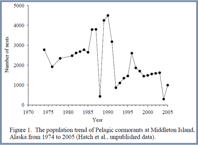
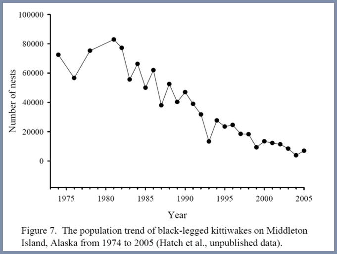
Random variables

Environmental stochasticity

Demographic stochasticity

Random variables

A random variable is a variable whose value can’t be predicted with certainty.

Examples

• Weather
• Our own behavior
• Population size

Is the universe random? Or is just too complex to be predicted with certainty?

Probability distributions

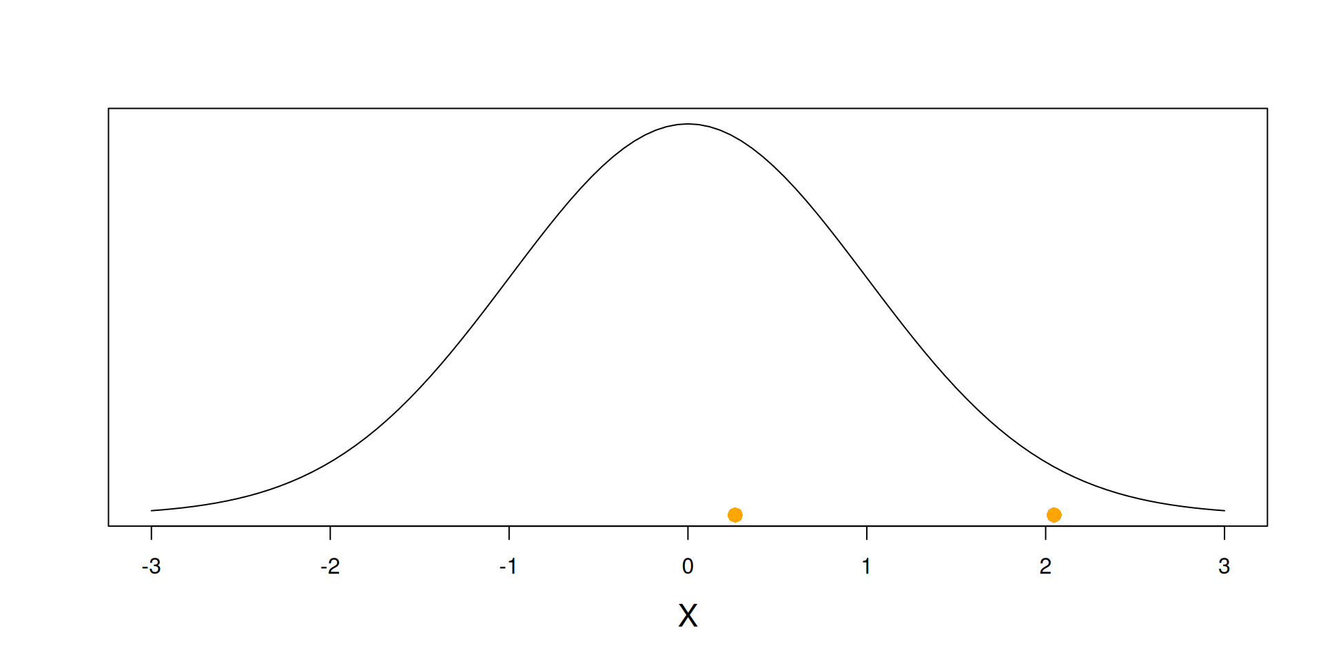
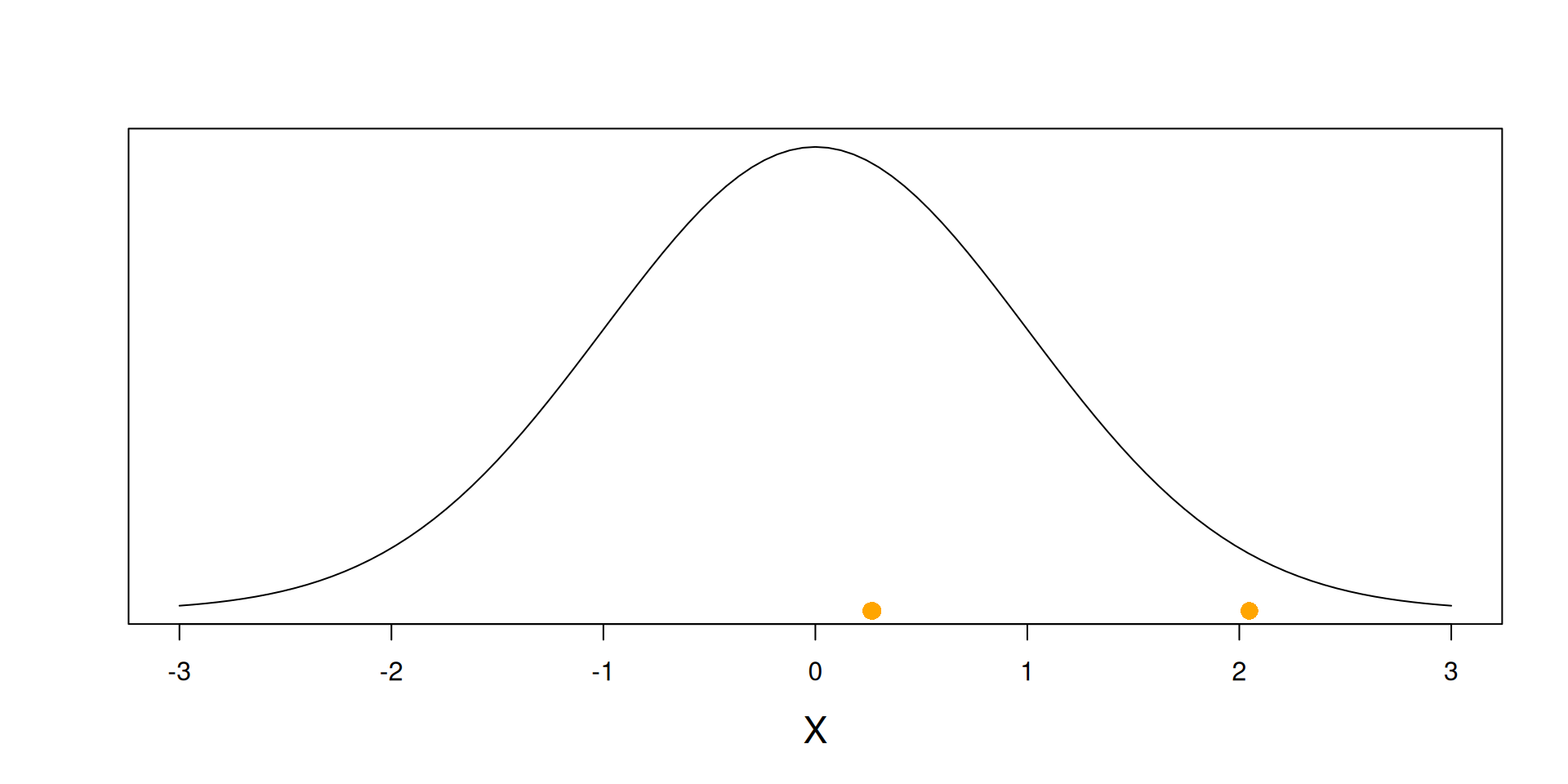
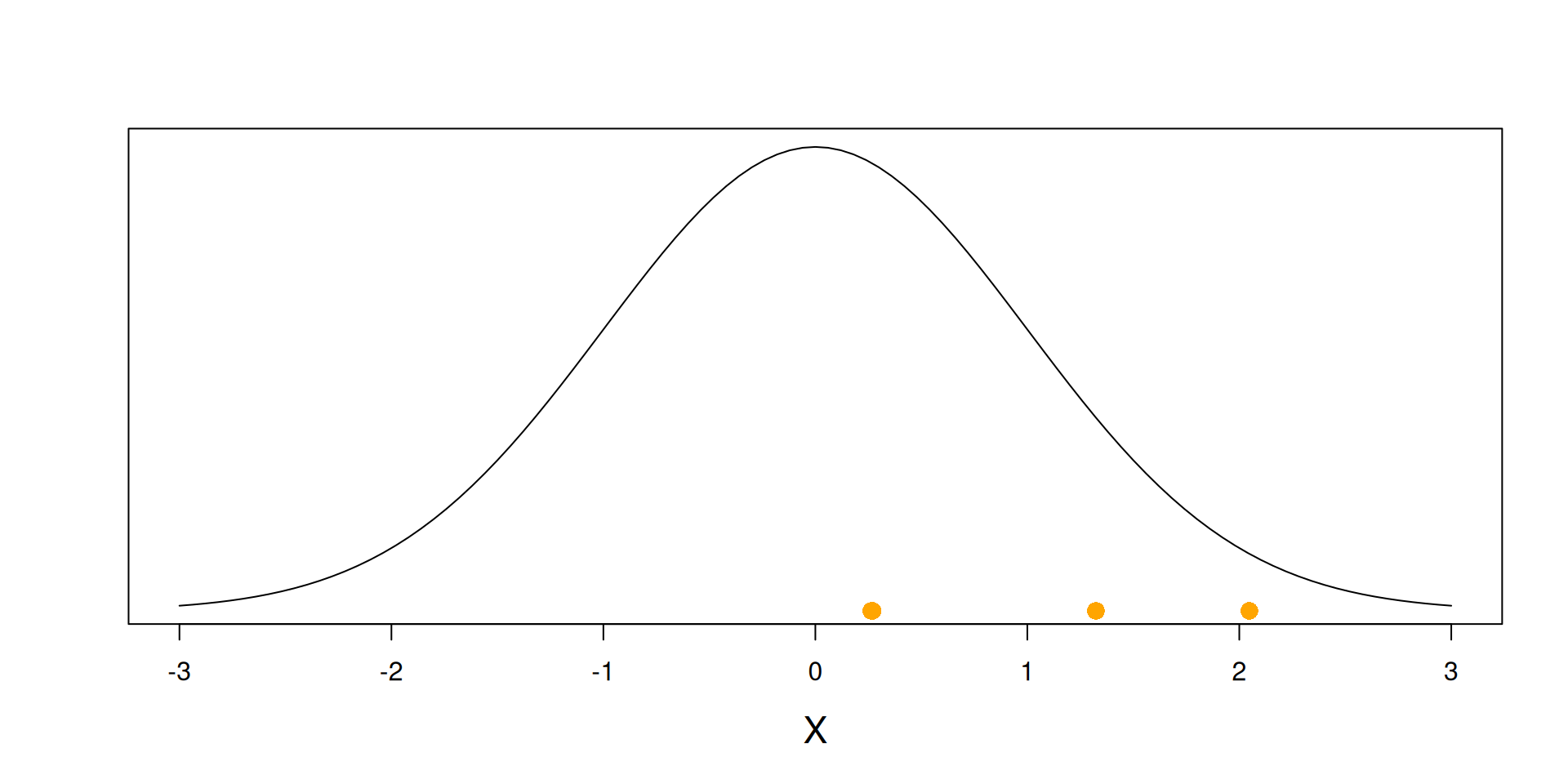
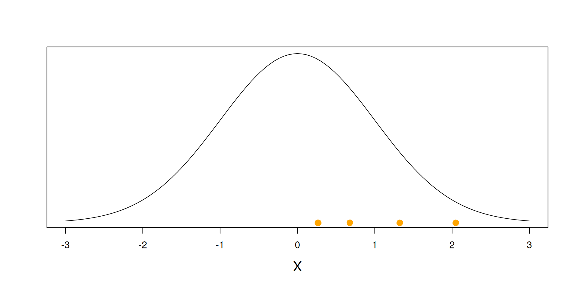
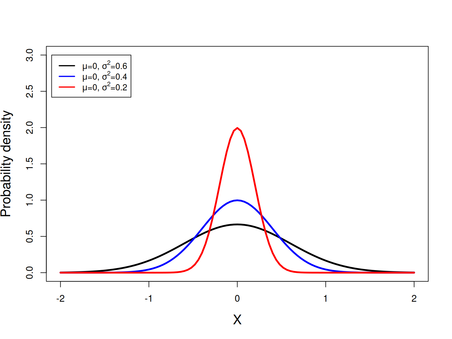
A random variable (\(X\)) can be described by a probability distribution.

There are many types of probability distributions, including:

• Normal (or Gaussian)
• Poisson
• Binomial
• Multinomial

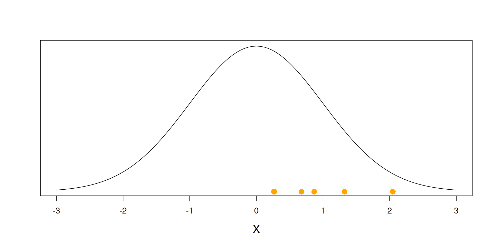
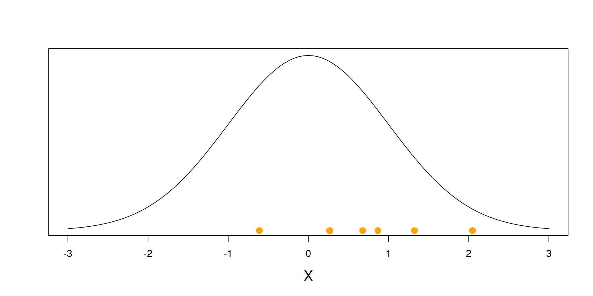
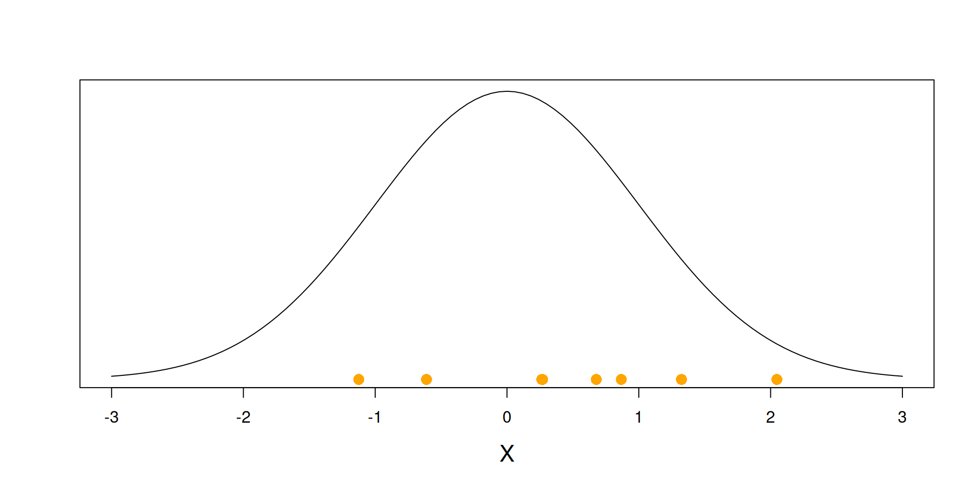
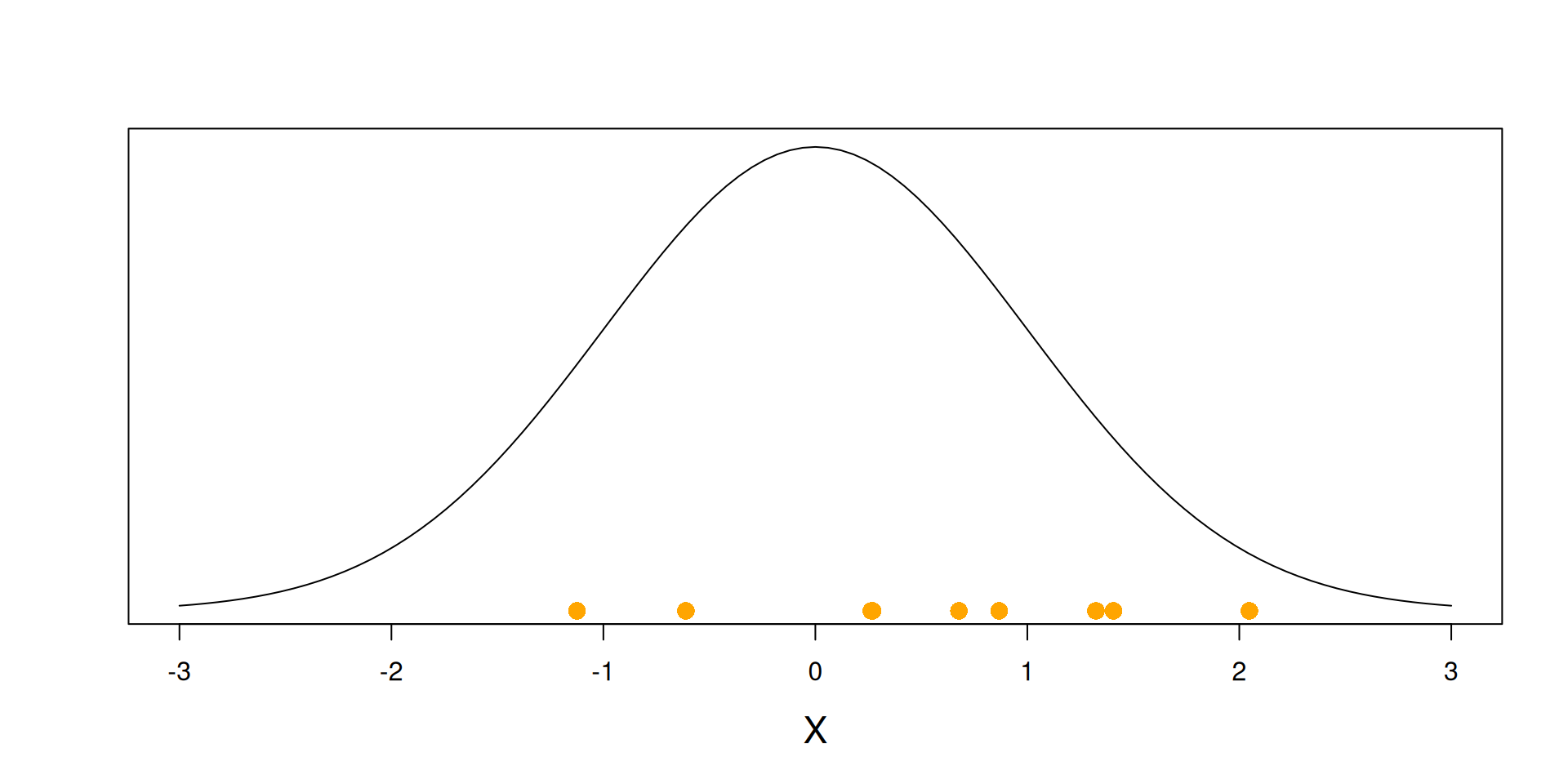
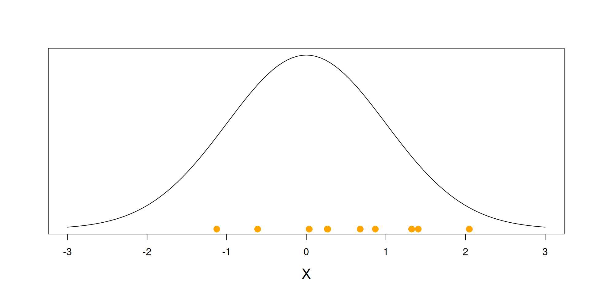
Normal (Gaussian) Distribution

\[ X \sim \mbox{Normal}(\mu=0, \sigma^2=1) \]

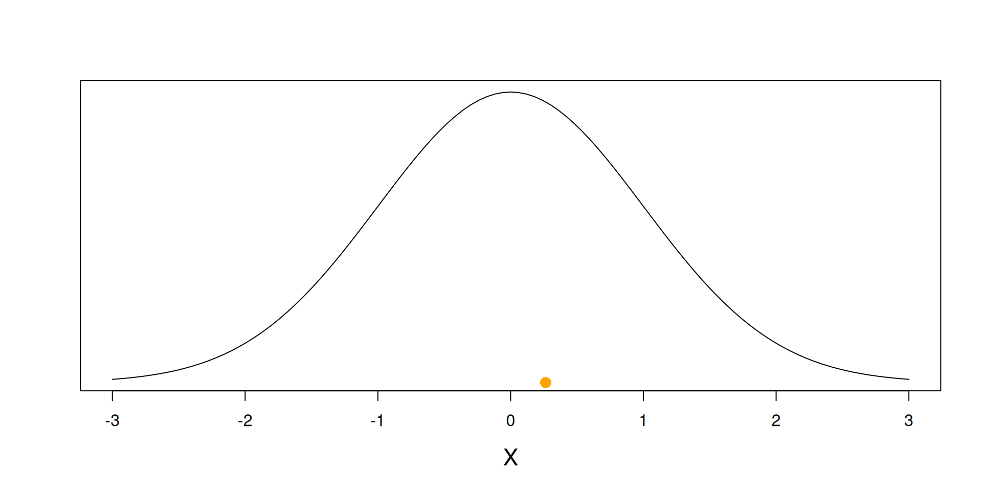
Normal (Gaussian) distribution

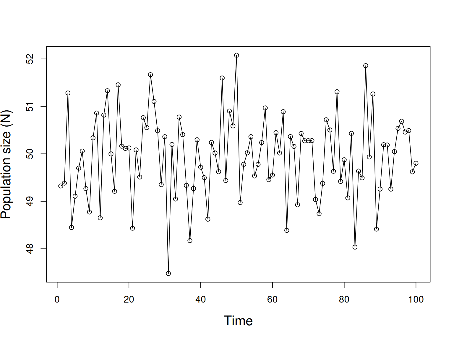
A purely stochastic model

\[ N_t \sim \mbox{Normal}(\mu=50, \sigma^2=1) \]

Two important types of stochasticity

Environmental stochasticity

• Random variation in demographic rates (such as birth and death rates).
• Caused by unpredictable changes (e.g., in weather, habitat, … conditions) among years.

Demographic stochasticity

• Random variation in demographic outcomes (such as the number of births and deaths).
• Occurs even when demographic rates are constant.

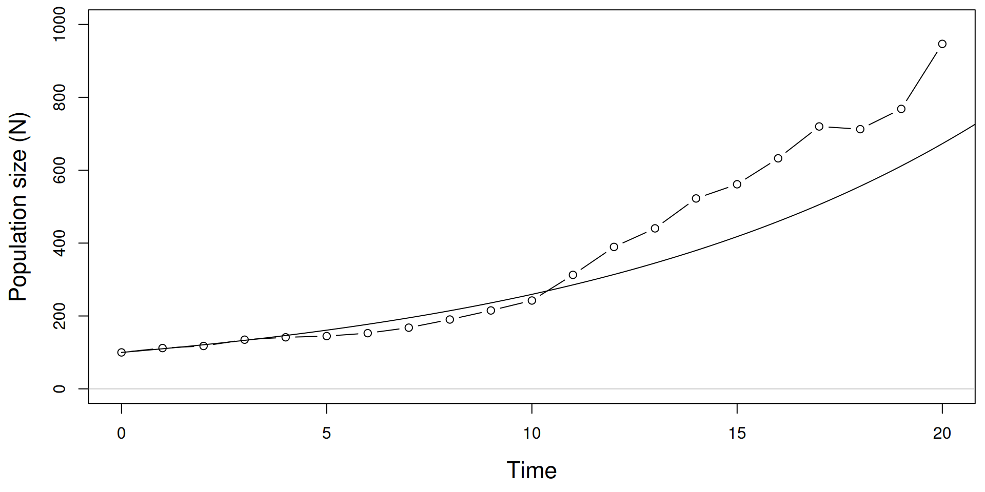
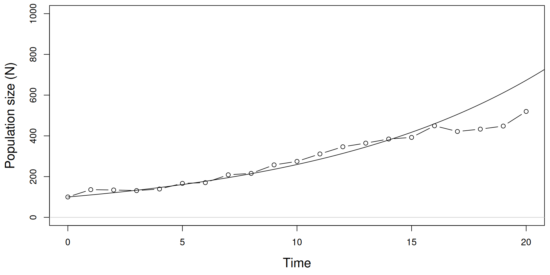
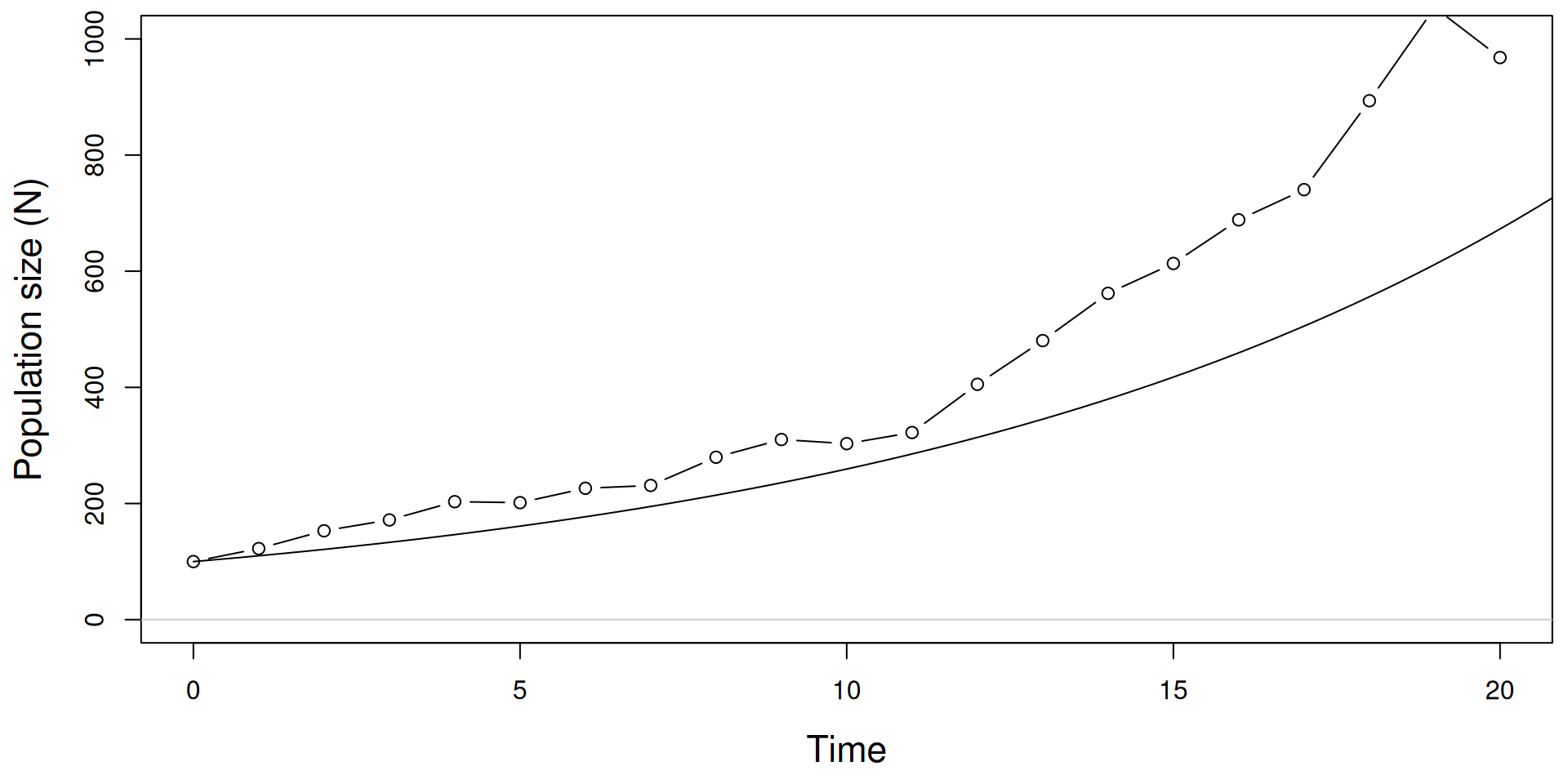
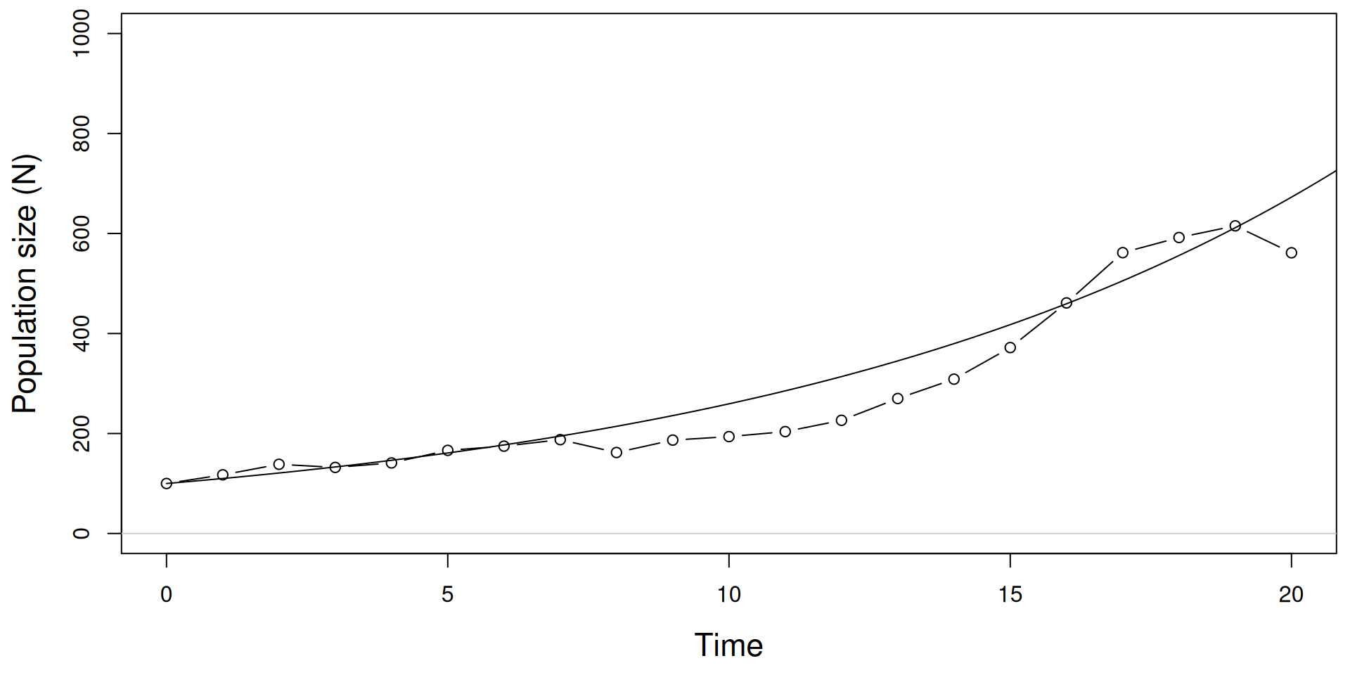
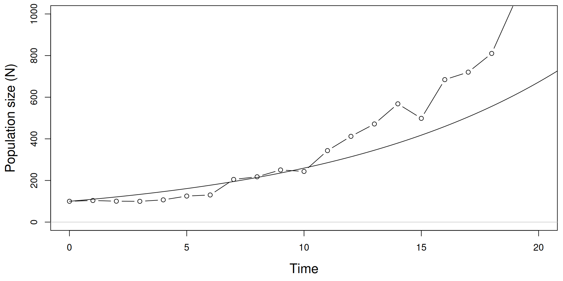
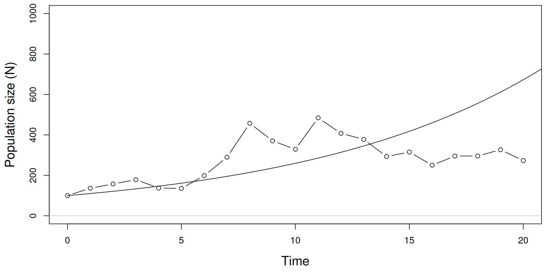
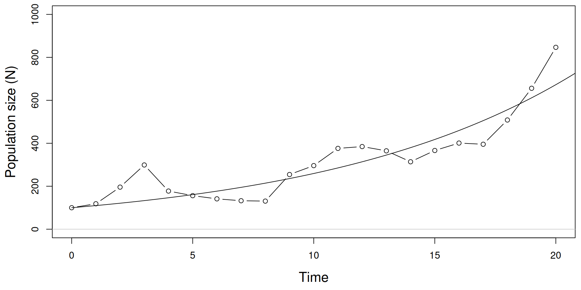
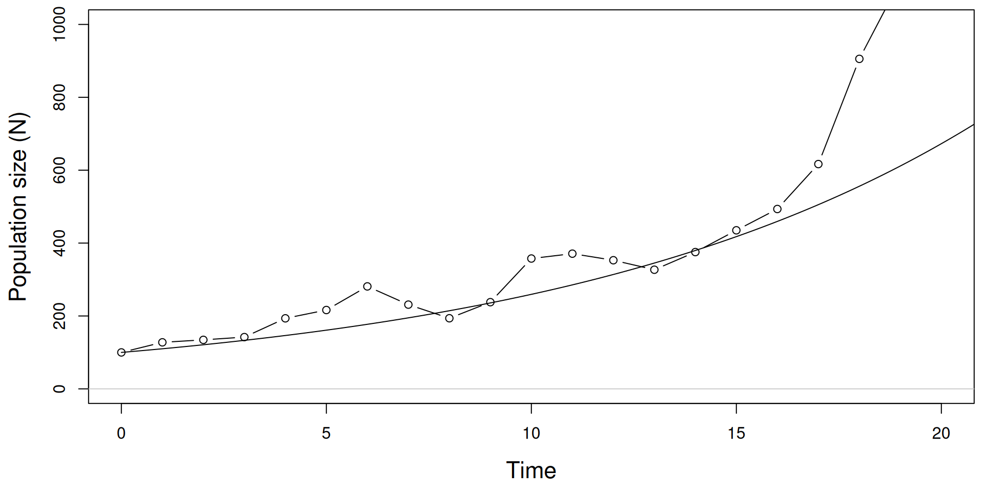
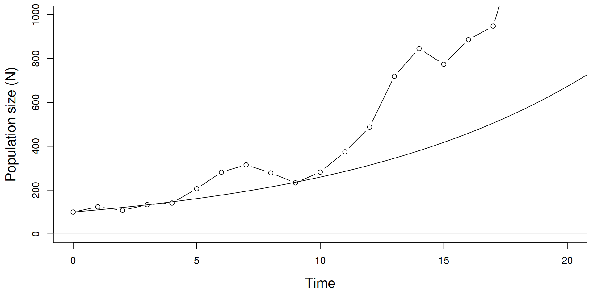
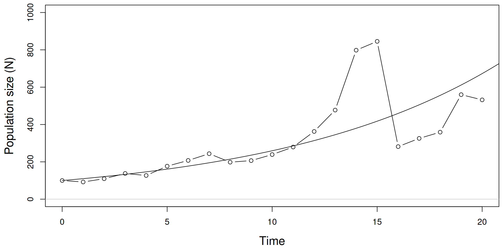
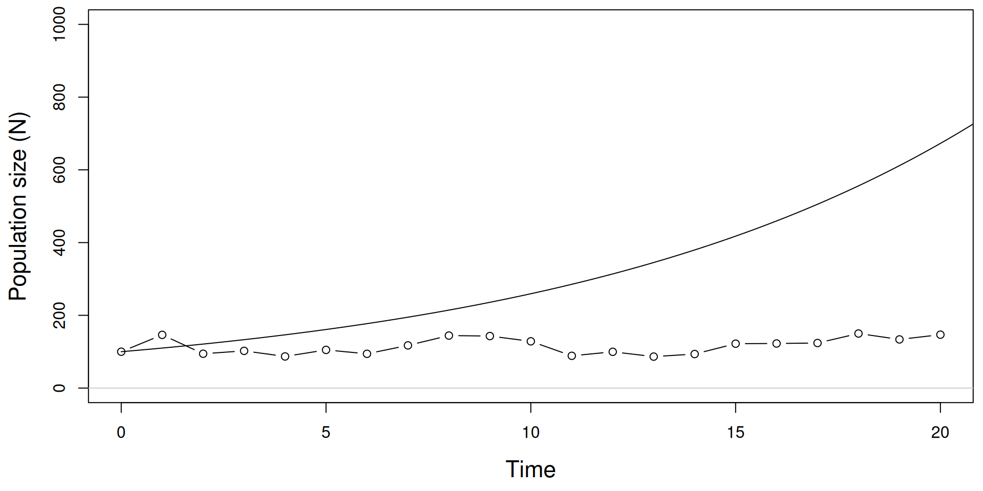
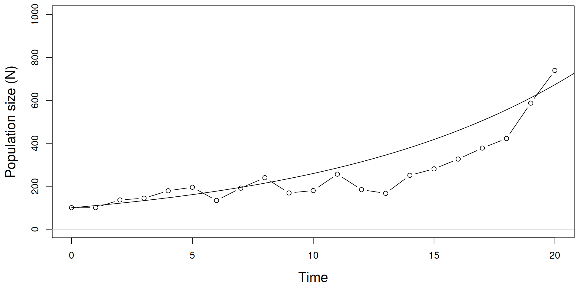
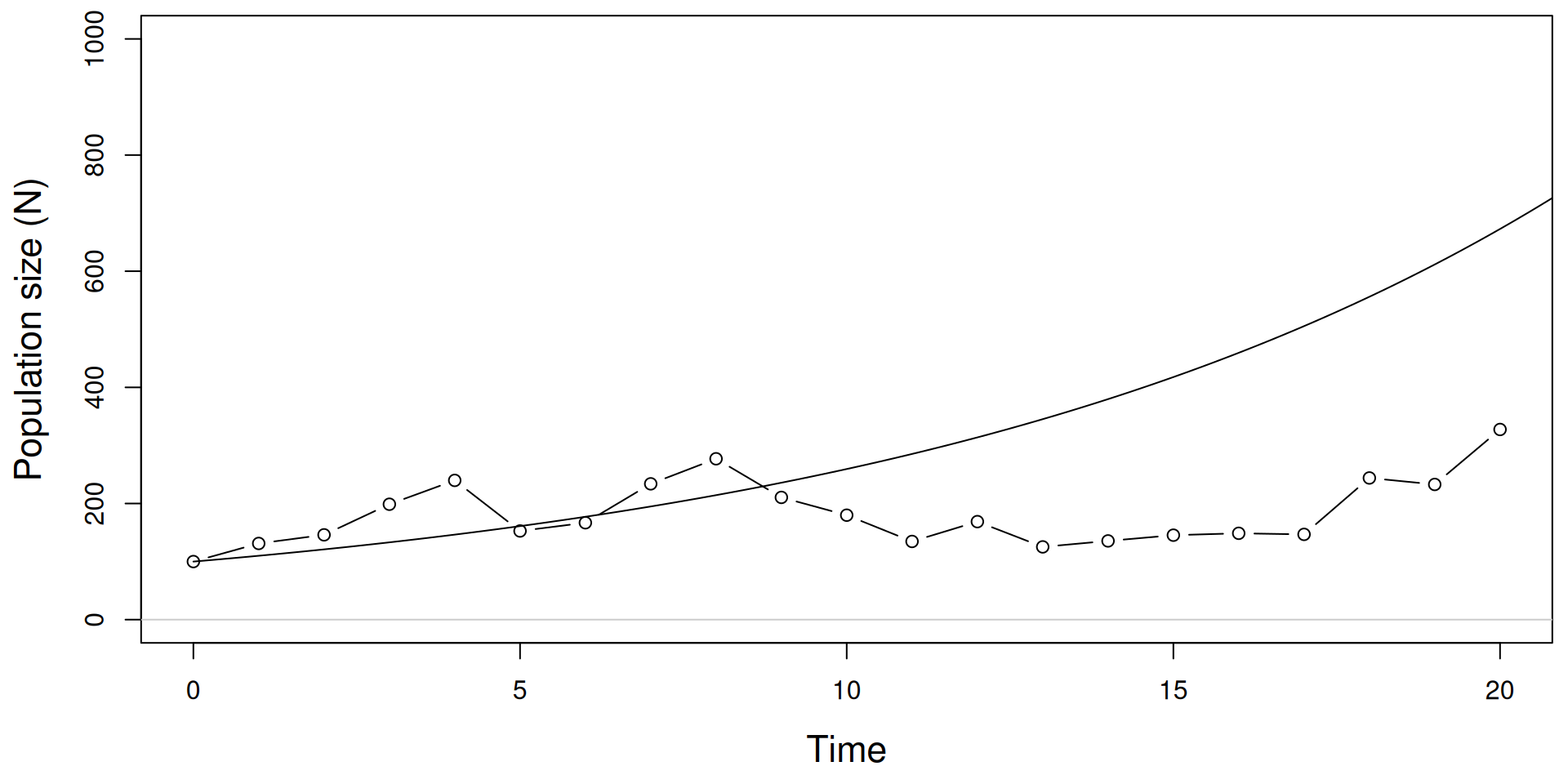
Geometric growth with env. stochasticity

\[ N_{t+1} = N_t + N_t r_t \]

\[ r_t \sim \mbox{Normal}(\bar{r}, \sigma^2) \]

R code

nYears <- 20
N <- r <- rep(NA, nYears)  ## Create empty N and r
N[1] <- 100                ## Initial value of N
r.bar <- 0.5               ## Average growth rate
sigma <- 0.1               ## StdDev of growth rate
for(t in 2:nYears) {
    r[t-1] <- rnorm(n=1, mean=r.bar, sd=sigma)
    N[t] <- N[t-1] + N[t-1]*r[t-1]
}

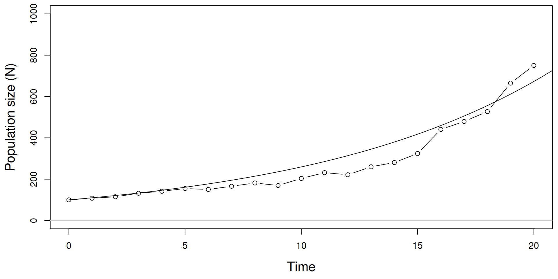
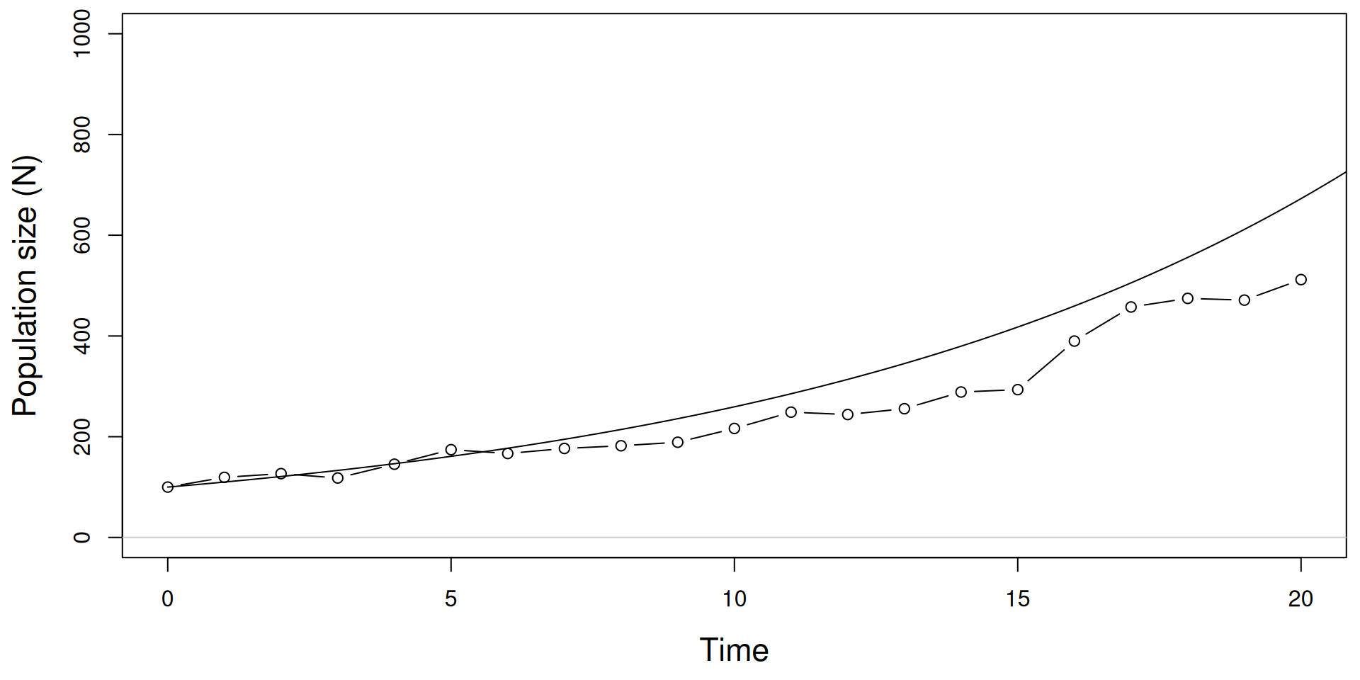
Geometric growth with env. stochasticity

\[ r_t \sim \mbox{Normal}(\bar{r}=0.1, \sigma^2=0.01) \]

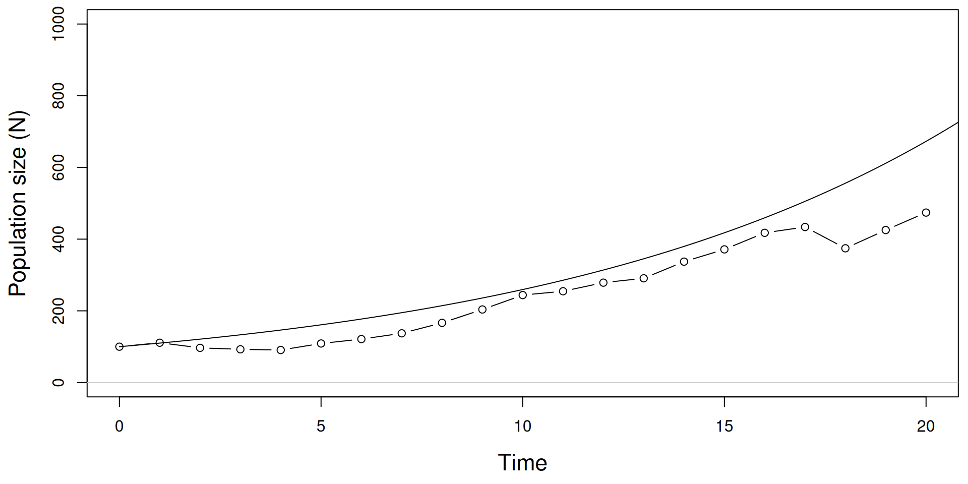
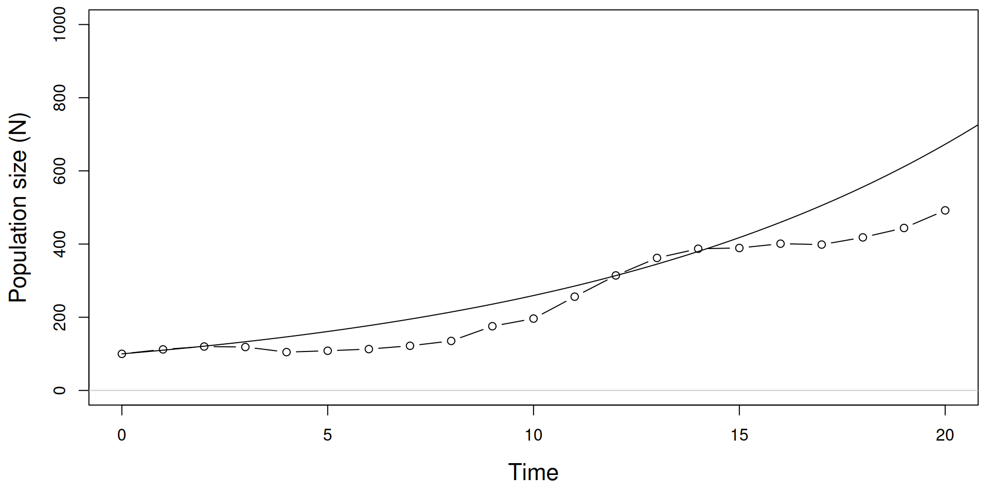
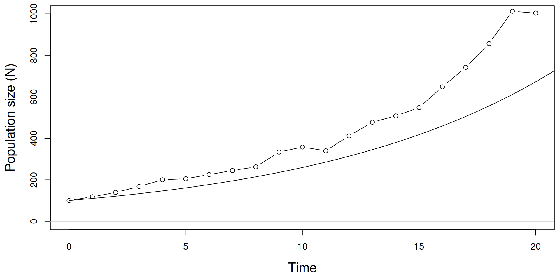
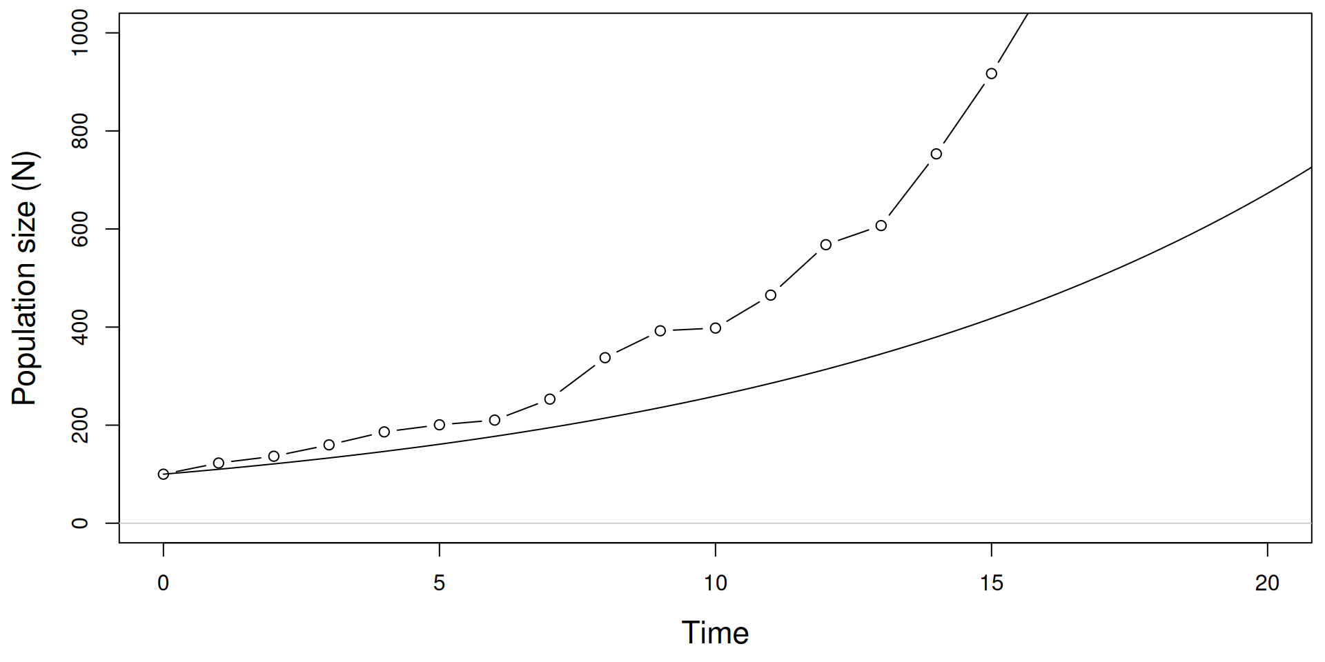
Geometric growth with env. stochasticity

\[ r_t \sim \mbox{Normal}(\bar{r}=0.1, \sigma^2=0.25) \]

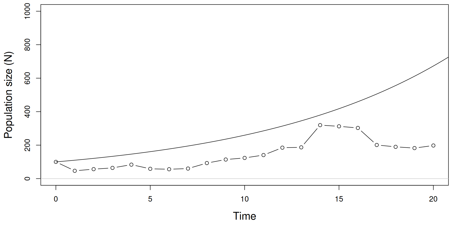
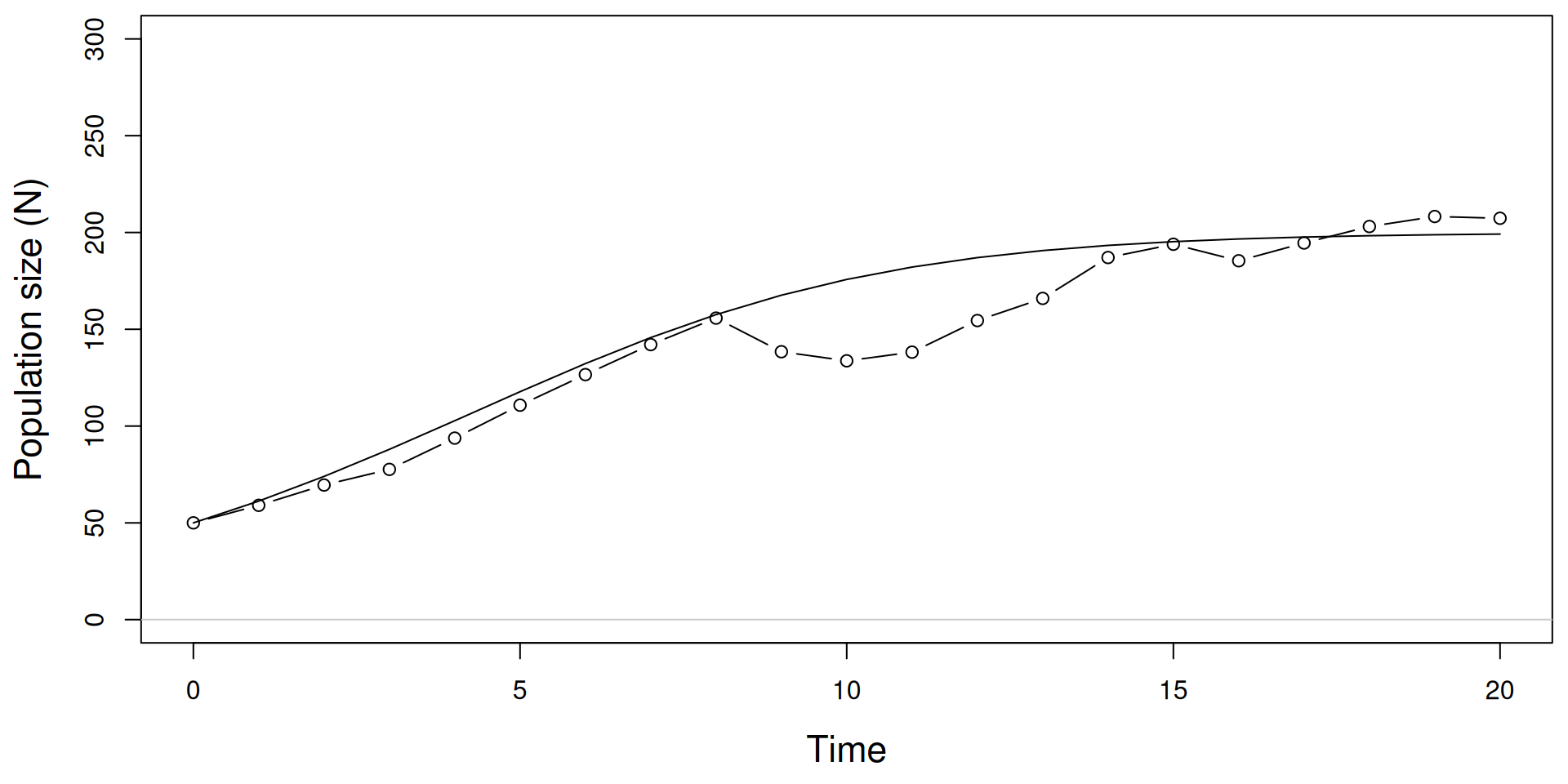
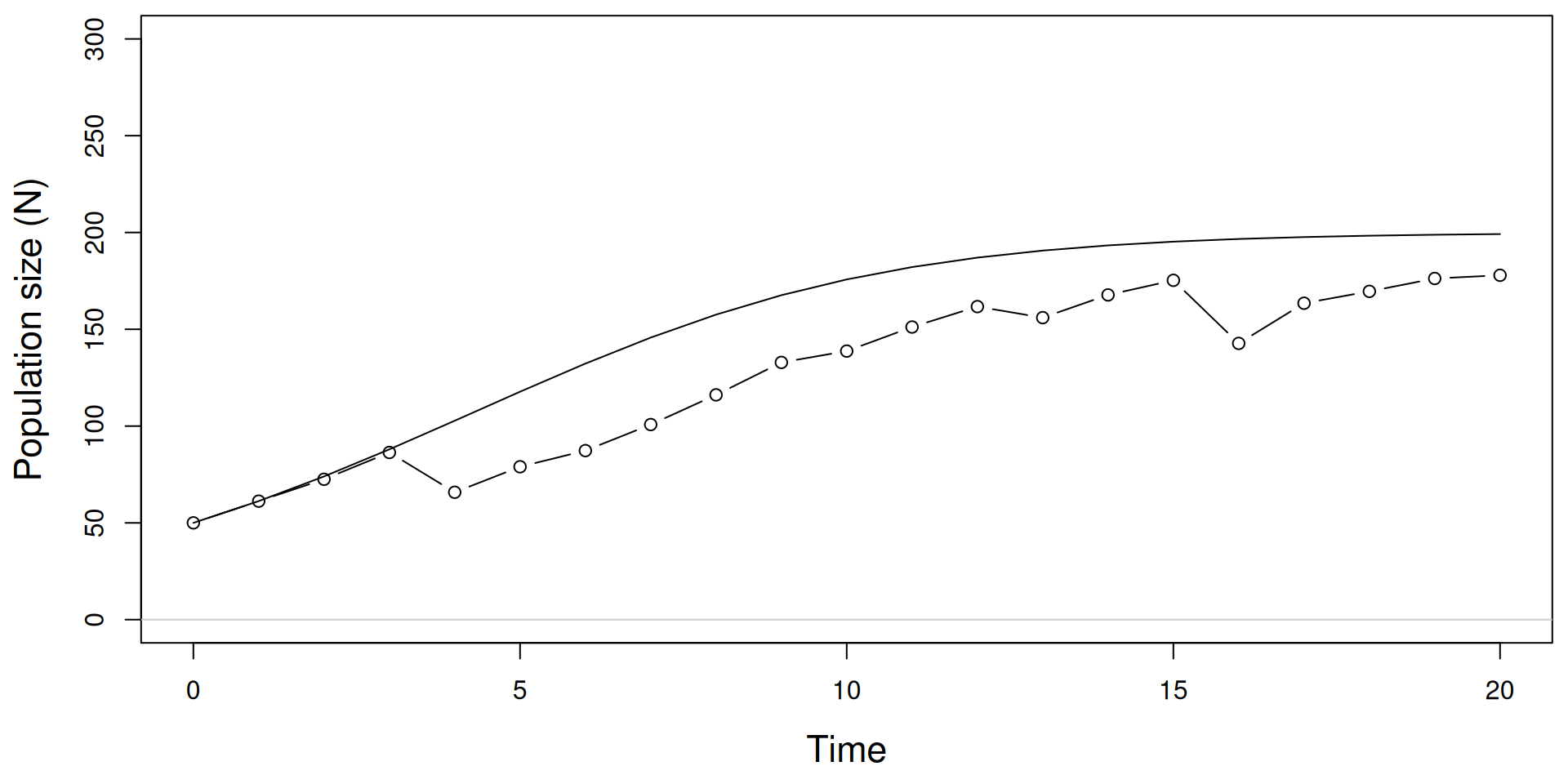
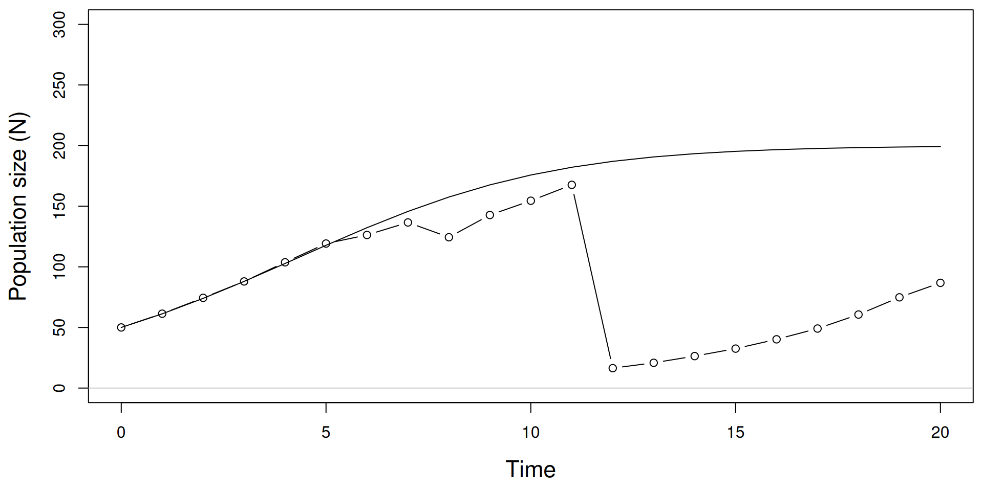
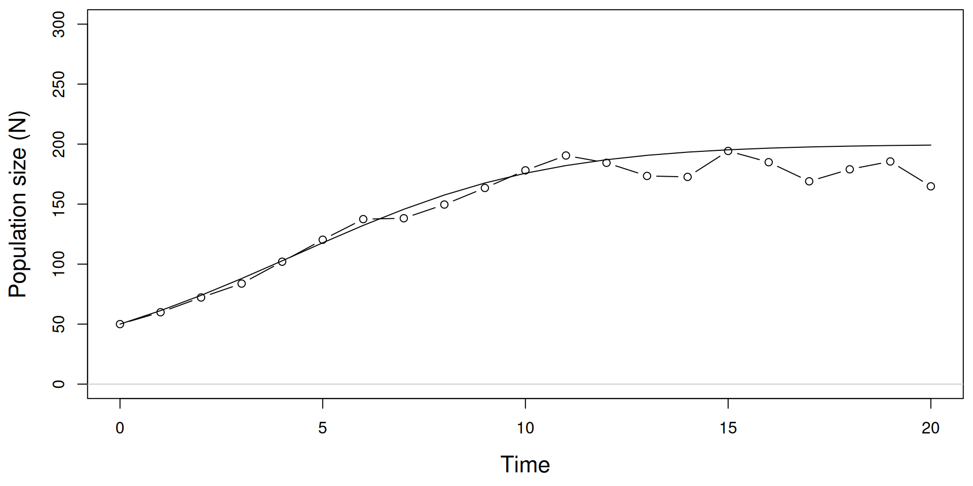
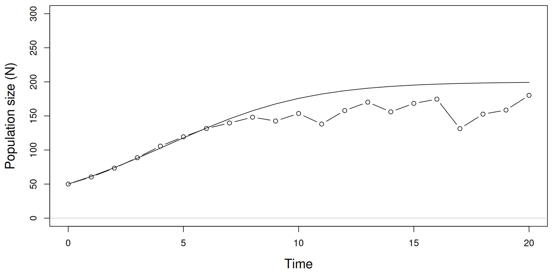
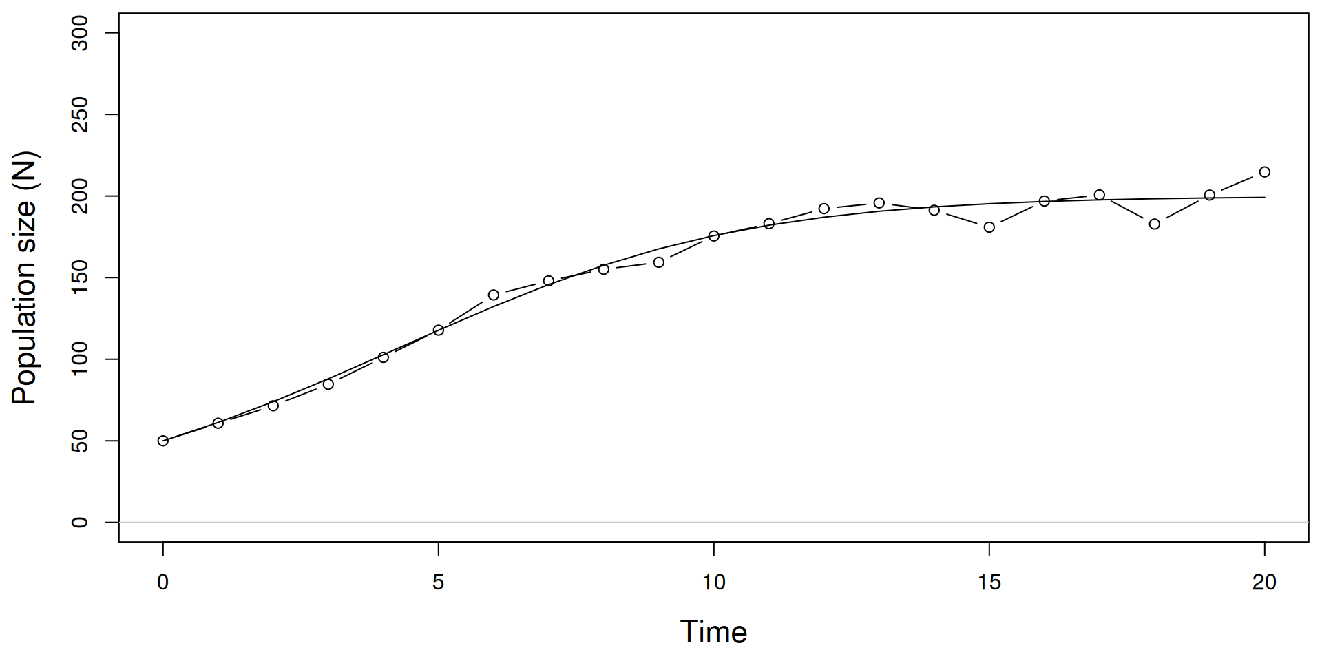
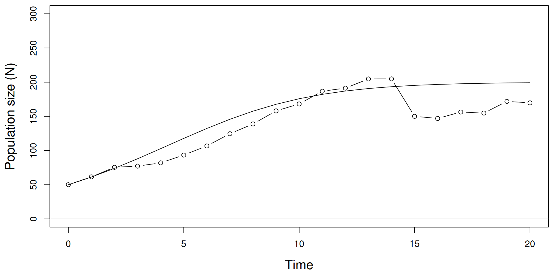
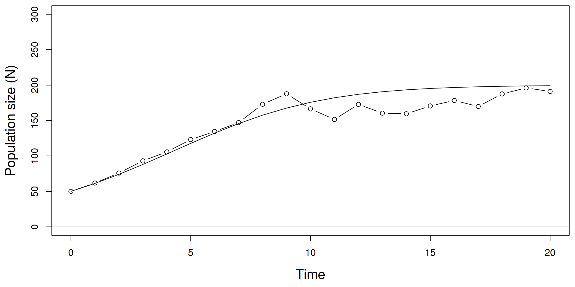
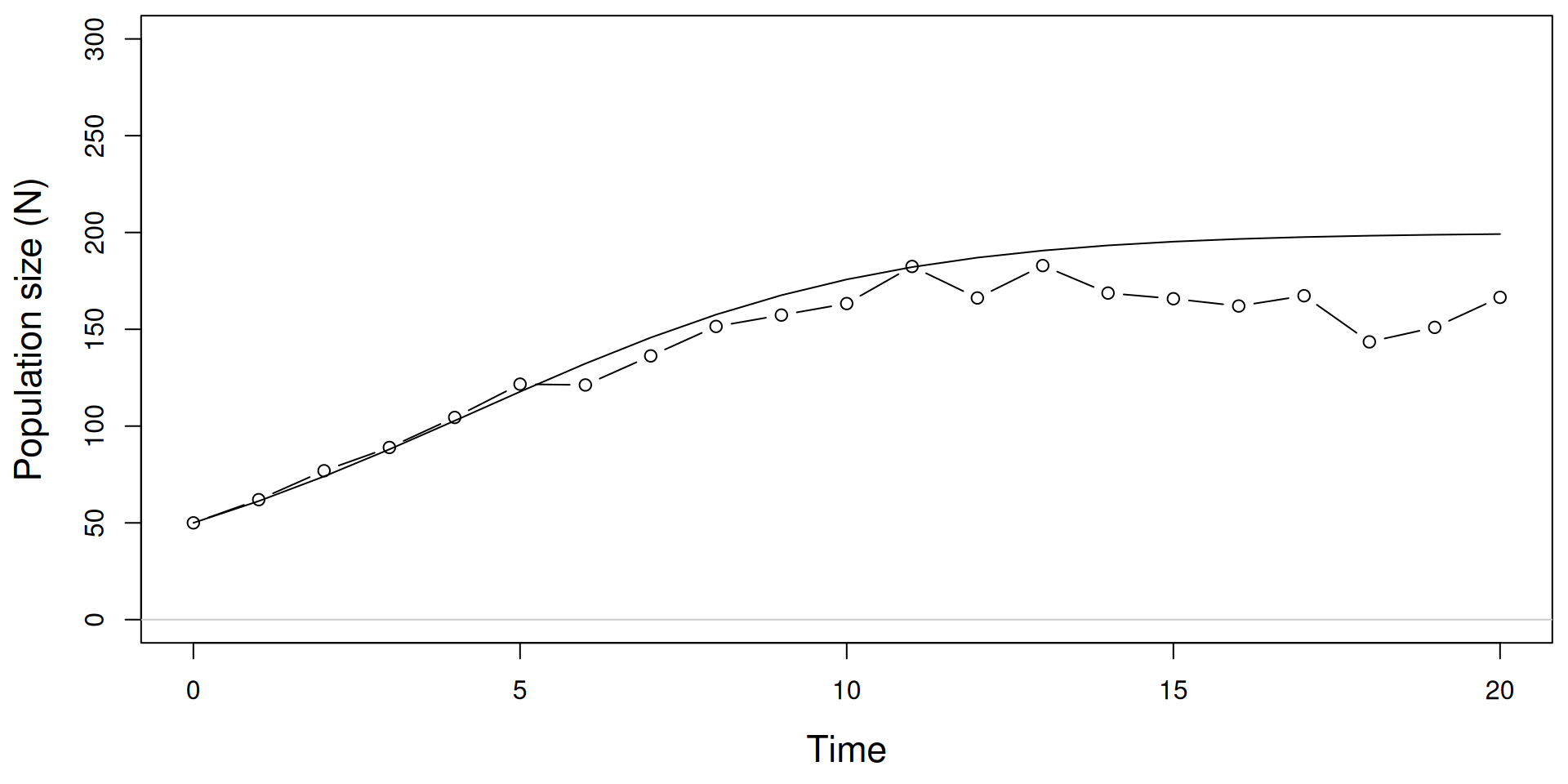
Logistic growth with environmental stochasticity

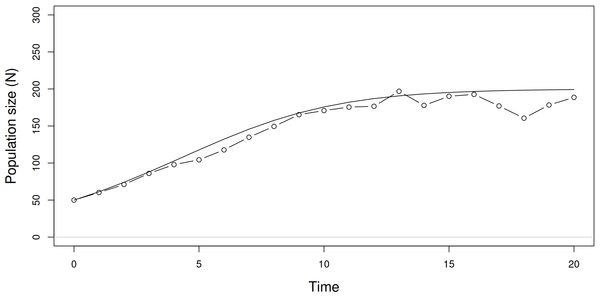
Imagine the carrying capacity fluctuates randomly.

\[ N_{t+1} = N_t + N_tr_{max}(1 - N_t/K_t) \\ K_t \sim \mbox{Normal}(\bar{K}, \sigma^2) \]

Logistic example with environmental stochasticity

\[ K_t \sim \mbox{Normal}(\bar{K}=200, \sigma^2=50) \]

Demographic stochasticity

We can make the BIDE model stochastic by modeling random variation in the number of individuals that are born and die each year (we’ll ignore movement):

\[ N_{t+1} = N_t + B_t - D_t \]

What distributions should we use for \(B_t\) and \(D_t\)?

\[ B_t \sim \mathrm{Poisson}(N_t\times b) \] \[ D_t \sim \mathrm{Binomial}(N_t, d) \]

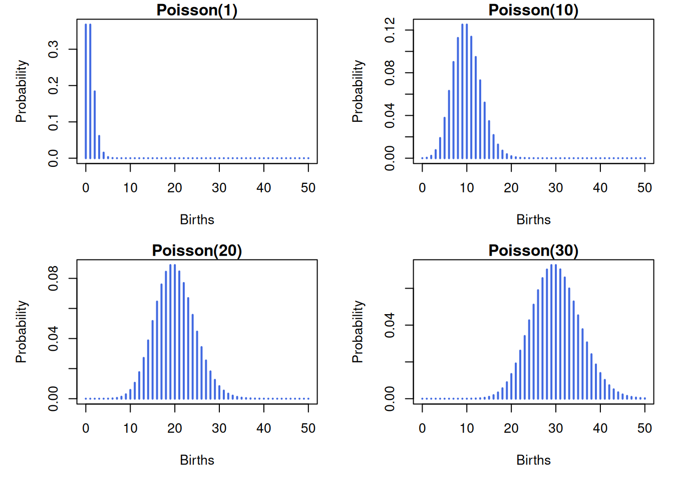
Poisson distribution

The Poisson distribution is useful for data that are non-negative integers.

It has a single parameter that describes the expected value of the random outcomes.

In stochastic population models, the Poisson distribution can be used to model the number of births (\(B_t\)) that occur in a time interval.

\[ B_t \sim \mathrm{Poisson}(N_t \times b) \]

Poisson distributions

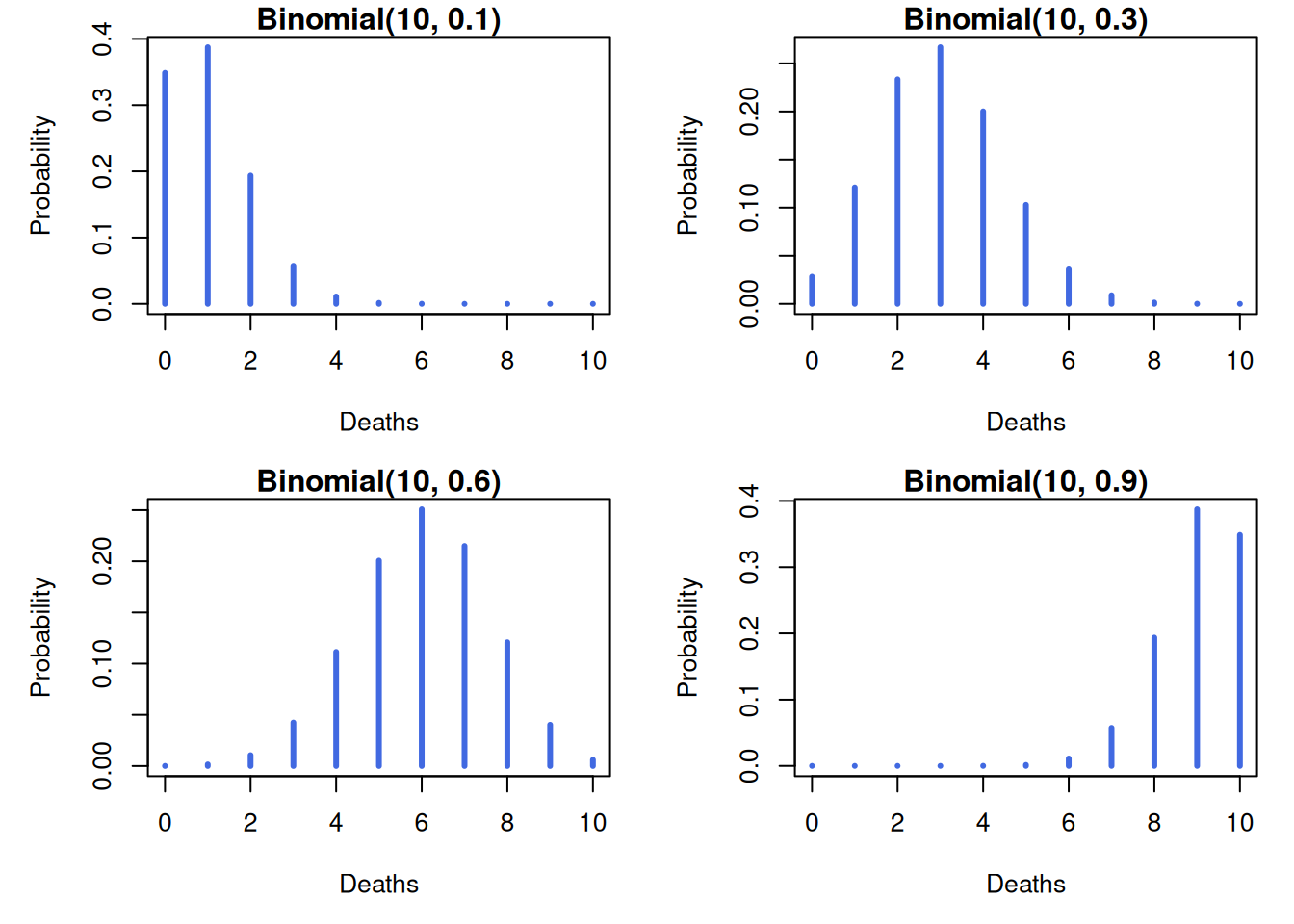
Binomial distribution

The binomial distribution is also useful for data that are non-negative integers, but it has an upper bound.

In population models, the upper bound is often population size, and we use the model to describe how many individuals die during some time period.

\[ D_t \sim \mathrm{Binomial}(N_t, d) \]

Binomial distributions

Demographic stochasticity

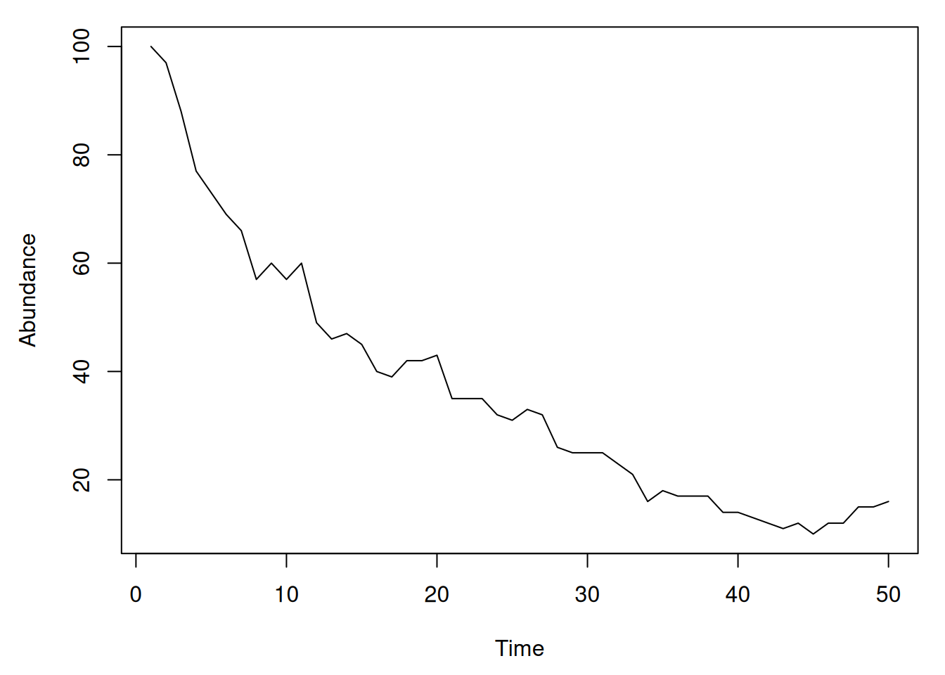
Poisson-Binomial birth-death model.

\[ \begin{gather*} N_{t+1} = N_t + B_t - D_t \\ B_t \sim \mathrm{Poisson}(N_t \times b) \\ D_t \sim \mathrm{Binomial}(N_t, d) \end{gather*} \]

Summary

Purely deterministic models are too rigid.

Purely stochastic models don’t describe population processes.

The goal is to develop mechanistic models that represent our biological understanding while allowing for uncertainty.