Parametric bootstrap method for fitted models inheriting class.

Simulate datasets from a fitted model, refit the model, and generate a sampling distribution for a user-specified fit-statistic.

Arguments

object	a fitted model inheriting class "unmarkedFit"
statistic	a function returning a vector of fit-statistics. First argument must be the fitted model. Default is sum of squared residuals.
nsim	number of bootstrap replicates
report	print fit statistic every 'report' iterations during resampling
seed	set seed for reproducible bootstrap
parallel	logical (default = `TRUE`) indicating whether to compute bootstrap on multiple cores, if present. If `TRUE`, suppresses reporting of bootstrapped statistics. Defaults to serial calculation when `nsim` < 100. Parallel computation is likely to be slower for simple models when `nsim` < ~500, but should speed up the bootstrap of more complicated models.
ncores	integer (default = one less than number of available cores) number of cores to use when bootstrapping in parallel.
...	Additional arguments to be passed to statistic

Details

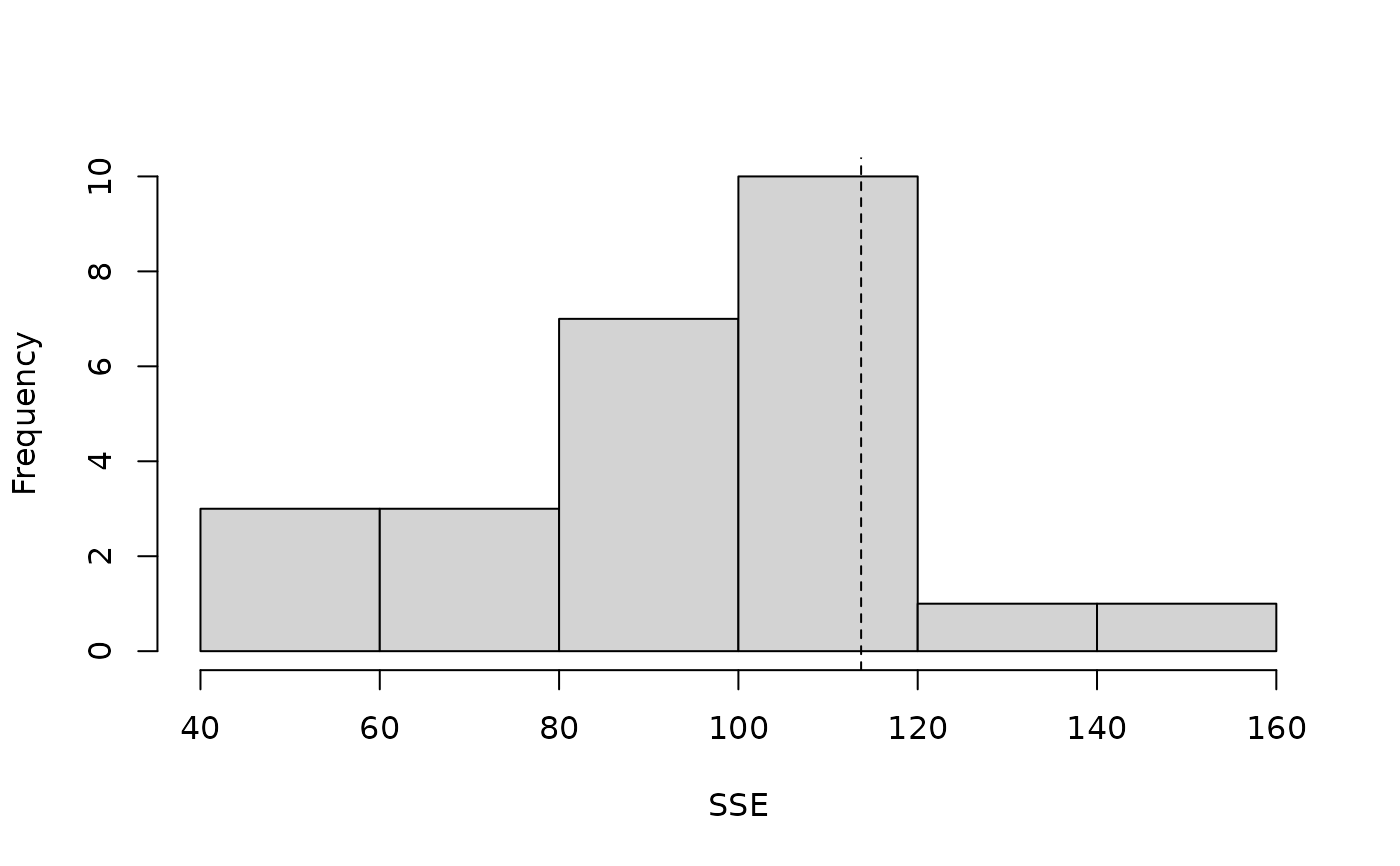
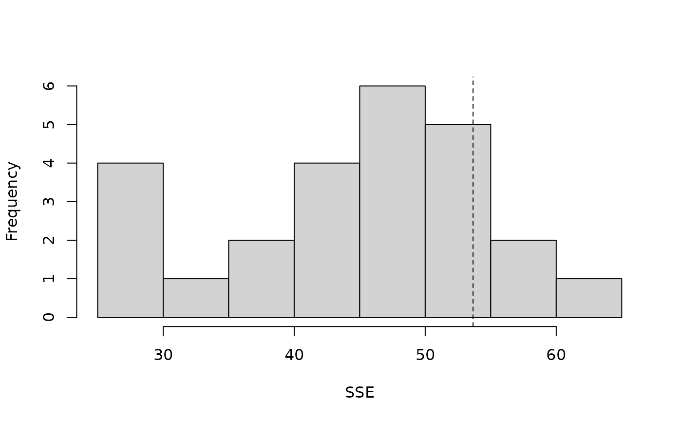
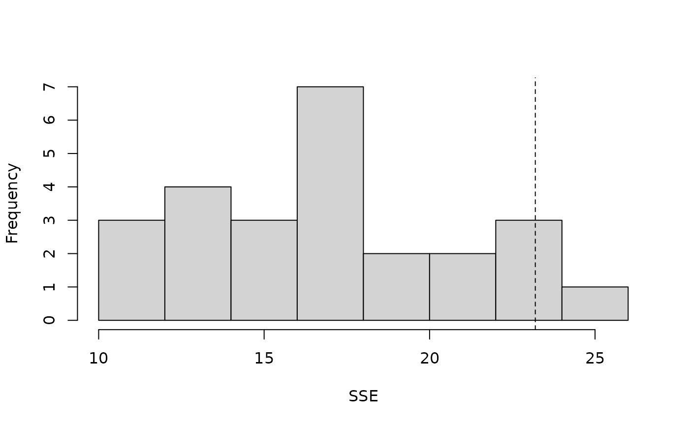
This function simulates datasets based upon a fitted model, refits the model, and evaluates a user-specified fit-statistic for each simulation. Comparing this sampling distribution to the observed statistic provides a means of evaluating goodness-of-fit or assessing uncertainty in a quantity of interest.

Value

An object of class parboot with three slots:

call

parboot call

Numeric vector of statistics for original fitted model.

t.star

nsim by length(t0) matrix of statistics for each simulation fit.

Author

Richard Chandler rbchan@uga.edu and Adam Smith

Examples


data(linetran)
(dbreaksLine <- c(0, 5, 10, 15, 20))
#> [1]  0  5 10 15 20
lengths <- linetran$Length

ltUMF <- with(linetran, {
  unmarkedFrameDS(y = cbind(dc1, dc2, dc3, dc4),
  siteCovs = data.frame(Length, area, habitat), dist.breaks = dbreaksLine,
  tlength = lengths*1000, survey = "line", unitsIn = "m")
    })

# Fit a model
(fm <- distsamp(~area ~habitat, ltUMF))
#> 
#> Call:
#> distsamp(formula = ~area ~ habitat, data = ltUMF)
#> 
#> Density:
#>             Estimate    SE     z P(>|z|)
#> (Intercept)   -0.287 0.167 -1.72  0.0852
#> habitatB       0.253 0.198  1.28  0.2000
#> 
#> Detection:
#>             Estimate    SE     z  P(>|z|)
#> (Intercept)     3.06 0.548  5.57 2.53e-08
#> area           -0.13 0.096 -1.35 1.76e-01
#> 
#> AIC: 165.5482 

# Function returning three fit-statistics.
fitstats <- function(fm) {
    observed <- getY(fm@data)
    expected <- fitted(fm)
    resids <- residuals(fm)
    sse <- sum(resids^2)
    chisq <- sum((observed - expected)^2 / expected)
    freeTuke <- sum((sqrt(observed) - sqrt(expected))^2)
    out <- c(SSE=sse, Chisq=chisq, freemanTukey=freeTuke)
    return(out)
    }

(pb <- parboot(fm, fitstats, nsim=25, report=1))
#> t0 = 113.6884 53.6492 23.19506 
#> iter 1 :  51.76656 29.33734 12.13766 
#> iter 2 :  86.40796 47.36944 20.79663 
#> iter 3 :  101.0376 43.93918 17.6049 
#> iter 4 :  119.055 46.61317 18.78843 
#> iter 5 :  95.61046 46.82708 16.04149 
#> iter 6 :  117.9119 52.39022 17.77974 
#> iter 7 :  97.09245 48.89117 23.22477 
#> iter 8 :  132.7958 52.14974 17.68474 
#> iter 9 :  107.5958 46.70377 17.23415 
#> iter 10 :  73.06662 29.29117 11.18831 
#> iter 11 :  75.30468 37.47914 14.67528 
#> iter 12 :  115.3185 50.47065 22.94304 
#> iter 13 :  81.07769 40.60462 15.79172 
#> iter 14 :  112.6747 38.32514 13.14837 
#> iter 15 :  67.64564 45.55177 13.71304 
#> iter 16 :  42.77671 29.09115 13.11265 
#> iter 17 :  80.65436 33.16117 11.87273 
#> iter 18 :  154.4764 60.23054 25.19856 
#> iter 19 :  104.4421 52.93641 23.86797 
#> iter 20 :  58.27236 29.40857 11.41073 
#> iter 21 :  100.7842 52.87954 18.40903 
#> iter 22 :  81.58062 41.29601 15.80306 
#> iter 23 :  118.4719 59.95035 21.71737 
#> iter 24 :  80.72755 43.11816 17.27023 
#> iter 25 :  104.6474 58.91896 17.89389 
#> 
#> Call: parboot(object = fm, statistic = fitstats, nsim = 25, report = 1)
#> 
#> Parametric Bootstrap Statistics:
#>                 t0 mean(t0 - t_B) StdDev(t0 - t_B) Pr(t_B > t0)
#> SSE          113.7          19.24            25.96        0.231
#> Chisq         53.6           8.97             9.58        0.115
#> freemanTukey  23.2           6.02             4.07        0.115
#> 
#> t_B quantiles:
#>              0% 2.5% 25% 50% 75% 97.5% 100%
#> SSE          43   48  81  97 113   141  154
#> Chisq        29   29  38  47  52    60   60
#> freemanTukey 11   11  14  17  19    24   25
#> 
#> t0 = Original statistic computed from data
#> t_B = Vector of bootstrap samples
#> 
plot(pb, main="")


# Finite-sample inference for a derived parameter.
# Population size in sampled area

Nhat <- function(fm) {
    sum(bup(ranef(fm, K=50)))
    }

set.seed(345)
(pb.N <- parboot(fm, Nhat, nsim=25, report=5))
#> t0 = 162.2135 
#> iter 5 :  151.6393 
#> iter 10 :  183.7412 
#> iter 15 :  156.2485 
#> iter 20 :  179.1255 
#> iter 25 :  135.8852 
#> 
#> Call: parboot(object = fm, statistic = Nhat, nsim = 25, report = 5)
#> 
#> Parametric Bootstrap Statistics:
#>    t0 mean(t0 - t_B) StdDev(t0 - t_B) Pr(t_B > t0)
#> 1 162          0.701             15.9        0.462
#> 
#> t_B quantiles:
#>      0% 2.5% 25% 50% 75% 97.5% 100%
#> t*1 129  132 151 162 174   184  184
#> 
#> t0 = Original statistic computed from data
#> t_B = Vector of bootstrap samples
#> 

# Compare to empirical Bayes confidence intervals
colSums(confint(ranef(fm, K=50)))
#>  2.5% 97.5% 
#>   117   218